Weather and climate vary on a range of time scales: from short term weather to climatic changes that happened over thousands or millions of years. A schematic diagram of the different time scales and constraining factors is shown below.
Source: International Institute for Sustainable Development/World Meteorological Organization
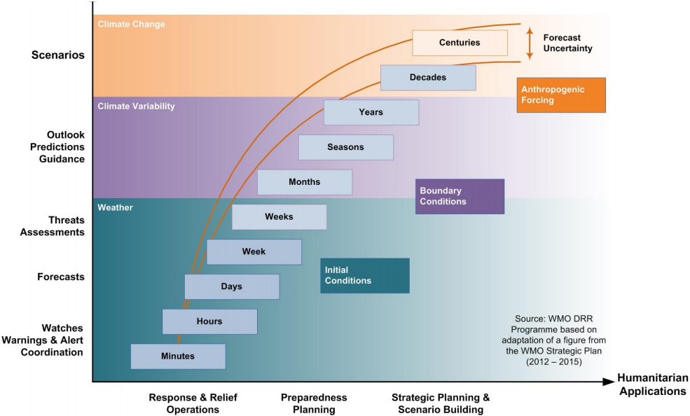
The forecast skill that exists at these time scales can be summarized by the graphic below.
Source: International Research Institute for Climate and Society

Weather
The term weather generally refers to the evolution of atmospheric conditions (temperature, precipitation, cloudiness, windiness, etc.) on a time scale up to about 10 days to two weeks. Considerable advances have been made in this field over the last century and weather forecasting skill in many regions of the world is quite good. The science of predicting weather is discussed in more detail in the more technical discussion on the Forecasting and Downscaling Methods page. But in essence, weather prediction constitutes using highly detailed observations and the framework of the Navier-Stokes equations of fluid motion to resolve how the atmosphere is likely to evolve in the coming days to two weeks. The main constraint on forecast skill is the accuracy and granularity of the initial conditions.
Weather forecasts typically give a forecast expected high and low temperature for each day and make a forecast of which days in the coming week and a half or two are likely to experience what form of precipitation, in what amounts and what level of wind is expected. As shown above, weather forecast skill tends to diminish in the one week to two week range.
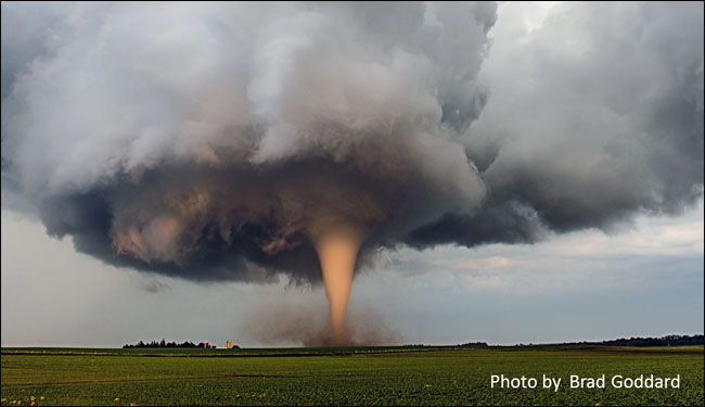
For really severe events (severe winter storms, hurricanes/cyclones, derechos and squalls, tornadoes and severe thunderstorms with lightning and hail), it is especially critical for weather services to provide and accurate and timely forecast of the conditions and the timing of the worst impacts. Offering such refined temporal and spatial information rapidly and accurately can save many lives in the context of a natural disaster.
National meteorological or weather services around the world are tasked with the responsibility of making daily and weekly weather forecasts and perform this task using numerical weather prediction methods and computer models. Some of the most prominent weather models in common use are the Global Forecast System (GFS) model produced by the National Center for Environmental Prediction (NCEP) within the US National Oceanic and Atmospheric Administration (NOAA), the Weather Research and Forecasting (WRF) model produced by the University Corporation for Atmospheric Research (UCAR) and the European Center for Medium Range Weather Forecasting (ECMWF) model.
Here are links to some prominent National and International Weather Services:
USA – National Weather Service
World Meteorological Organization Weather Mandate
Weather and Climate Modeling
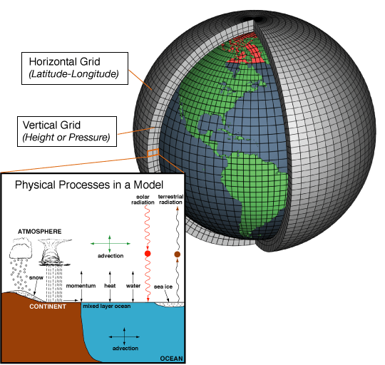
Both weather and climate modeling involve dividing the world’s surface, atmosphere and ocean into a fine network of gridboxes (in both horizontal and vertical dimensions), for which the equations of motion, heating, radiation, relative humidity and surface hydrology are evaluated. The spatial and temporal resolution of these models depends on the specific model and application, but the overall schematic is depicted below. These models are fed continuous observations from satellites and stations and programmed to apply the governing equations of the atmosphere to make predictions.
source: https://celebrating200years.noaa.gov/breakthroughs/climate_model/modeling_schematic.html
The temporal frequency of inputs used for climate modeling is more limited than the temporal frequency of inputs used for weather modeling. The spatial resolution of the gridboxes in global climate models (GCMs) is also more limited than is typically used to make weather forecasts. Weather forecasts are expected to produce highly temporally and spatially resolved forecasts, but usually over a smaller region. Global climate models are tasked with understanding forecast and projected changes in global patterns of weather and climate. While there are many climate modeling centers around the world, two of the major modeling collectives are the North American Multi-Model Ensemble (NMME) and the Copernicus (European) C3S. These are also archived on the IRI NMME and IRI Copernicus sites.
In addition to global climate models, there is sometimes a desire to run climate models at a higher resolution over a smaller domain using physically based regional climate models (RCMs). One of the more prominent RCM initiatives has been the COordinated Regional climate Downscaling EXperiment (CORDEX) initiative.
The science of weather and climate prediction has improved considerably since the early to mid 20th century, thanks in part to important conceptual discoveries, tremendous improvements in computational power and the much wider array of observational data available today to inform our understanding of the planet. Significant challenges still remain though, particularly at the sub-seasonal, decadal and longer term climate change time scales.
Sub-seasonal Climate Variability
The term sub-seasonal climate variability is generally used to refer to variability on the time scale of two weeks to two months. This is a critically important time frame for many decisions across many sectors, but unfortunately, the skill of sub-seasonal predictability is less robust than that of weather forecasting or seasonal forecasting. This is still an active frontier in climate research. Rather than making specific predictions of temperature, precipitation, windiness or cloud cover on specific days, S2S forecasts often frame their conclusions in more general, probabilistic terms (eg. the third week from now is likely to be warmer and drier than normal (rather than Wednesday is predicted to have a high temperature of 25 C and be sunny)).
The two week+ time frame is too long to make the same kind of robust, granular forecasts that are possible at the weather time scale – because small differences in initial conditions diverge too much after two weeks. But the predictive information available from changing boundary conditions at this short time scale is usually less powerful than the predictive information available at a seasonal or interannual time scale. Nevertheless, S2S forecasts are made by both NMME and Copernicus and a number of other research centers around the world (including in Asia). One of the major global initiatives to understand S2S predictability is the S2S Prediction Project.
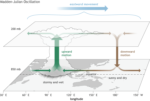
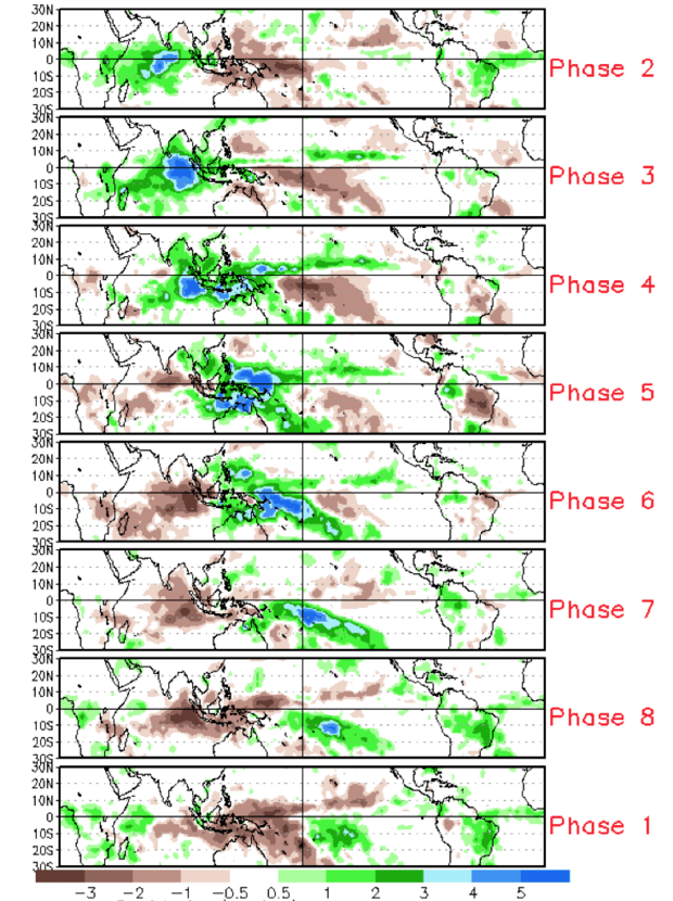
MJO: One of the main sources of S2S predictability is the Madden Julian Oscillation (MJO). The MJO is pattern of convection and subsidence in the global tropics that moves eastward over time and typically makes a full trip around the world on the time scale of 30-60 days. The schematic diagram and the typical rainfall anomalies associated with each of the 8 “phases” of the MJO are depicted below.
source: https://www.climate.gov/news-features/blogs/enso/what-mjo-and-why-do-we-care
BSISO: Another source of predictability at the subseasonal time scale is the Boreal Summer Intra-Seasonal Oscillation (BSISO). Like the MJO, this oscillation is analyzed in the context of 8 phases, but predominantly effects Southern and Eastern Asia and the Indo-Pacific region. More information is available on the Asia Pacific Economic Cooperation Climate Center (APEC CC or APCC) page.
Seasonal to Inter-annual Climate Variability
The term seasonal climate variability is generally used to refer to variability on the time scale from two months to the better part of a year and inter-annual variability refers to variability between consecutive years. There is a fair amount of predictive skill that exists for seasonal to interannual variability.
El Nino/Southern Oscillation (ENSO): One of the most prominent signals in the global climate system is the El Nino/La Nina phenomenon, also known as the El Nino-Southern Oscillation. A brief conceptual video is shown below:
ENSO animation from UK MetOffice
During the El Nino (warm) phase, easterly trade winds across the tropical Pacific weaken, sea surface temperatures in the Eastern tropical Pacific tend to be warmer and the center of convective rainfall shifts eastwards relative to neutral conditions. During the La Nina (cool) phase, the easterly trade winds intensify, sea surface temperatures in the Eastern tropical Pacific tend to be cooler and the center of convective rainfall shifts westwards relative to neutral conditions.
source: https://www.pmel.noaa.gov/elnino/schematic-diagrams

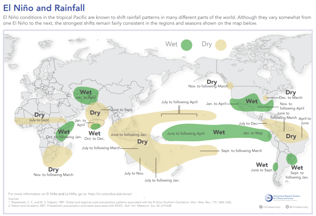
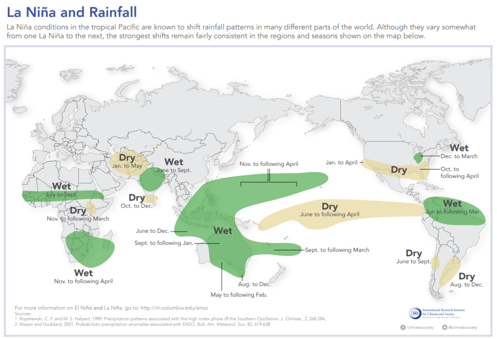
While the El Nino/La Nina phenomenon is centered in the tropical Pacific Ocean, it has global ramifications and alters the atmosphere-ocean dynamics around the world. There are number of well-understood and documented teleconnections to patterns of precipitation and temperature anomaly depending on the ENSO phase shown below:
Source: IRI
Impacts on the US are shown here
source: https://www.weather.gov/fwd/teleconnections
At present, (October 2023), the world is in a state of moderately strong El Nino. This is forecast to continue through early 2024. For more information, consult the NOAA Climate ENSO page.
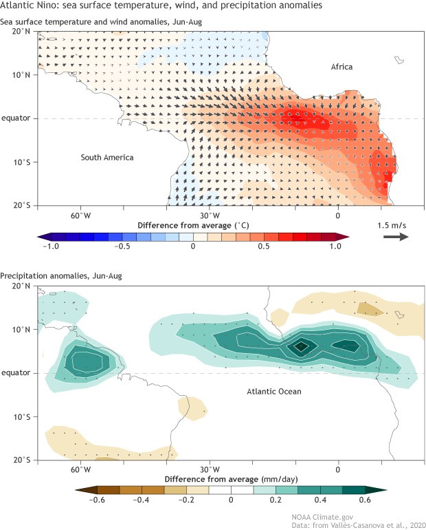
Atlantic NINO: While the El Nino pattern dominates both the Pacific basin and has global teleconnections, a similar pattern exists in the Atlantic – although the amplitude of the impacts on the local and global climate tend to be smaller (and tend to be confined to the Atlantic basin). During the “warm phase” of the Atlantic Nino pattern, sea surface temperatures in the Gulf of Guinea become anomalously warm leading to enhanced precipitation over that region, a general northward displacement of the ITCZ and some enhancement of precipitation to the north of the equator in South America (while simultaneously leading to suppressed rainfall in Brazil’s Nordeste region). This is depicted below.
During the “cool phase”, the opposite occurs and the waters of the Gulf of Guinea are cool and the coastal regions become drier and the ITCZ shifts southward and the Nordeste receives more rainfall.
For more information on this phenomenon, consult https://www.aoml.noaa.gov/the-atlantic-nino-el-ninos-little-brother/
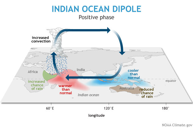
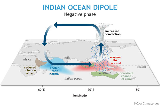
Indian Ocean Dipole: There is also a similar coupled oscillation pattern in the Indian Ocean, known as the Indian Ocean Dipole. During the warm or positive phase, the SSTs are warmer near the coast of East Africa and that region experiences enhanced rainfall, whereas the area around Indonesia and Australia experiences cooler SSTs and suppressed rainfall.
For more information on this phenomenon, consult https://www.climate.gov/news-features/blogs/enso/meet-enso%E2%80%99s-neighbor-indian-ocean-dipole
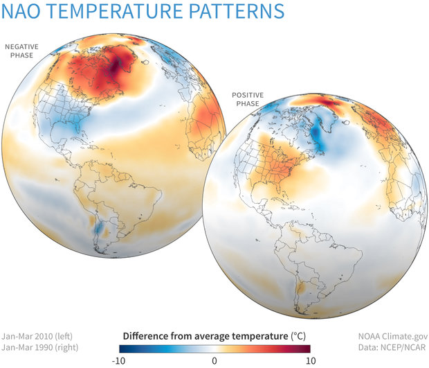
North Atlantic Oscillation: One of the dominant modes of seasonal variability (particularly in the winter time) in the northern hemisphere mid-latitudes and high latitudes is the North Atlantic Oscillation. The area around the Azores Islands off the coast of southern Europe and northern Africa typically experiences high atmospheric pressure, whereas the area near Iceland typically experiences low pressure.
When both of these pressure anomalies are stronger than normal, the NAO is said to be in the positive phase, which drives southwest to northeasterly flow from southeastern North America to northern Europe. This typically leads to warm wet winters in northern and central Europe and warm wet winters in the US East coast, but colder than normal conditions in Greenland and northeast Canada and a dry Mediterranean.
When both of these pressure anomalies are weaker than normal, the NAO is said to be in the negative phase which drives more west to east flow from central-eastern North America to the Mediterranean. This tends to lead to wetter than normal conditions in the Mediterranean, cold and dry conditions to northern Europe, colder conditions than normal in the eastern US and warmer than normal conditions in Greenland and northeast Canada.
source: https://www.ldeo.columbia.edu/res/pi/NAO/
positive phase precipitation effect
negative phase precipitation effect
source: https://www.climate.gov/news-features/understanding-climate/climate-variability-north-atlantic-oscillation
temperature patterns
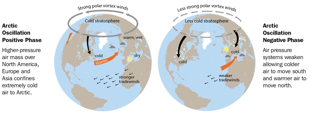
Arctic Oscillation: A closely related phenomenon is the Arctic Oscillation. In the “positive phase” the temperatures in the high Arctic are very cold, the surface pressure is low, the jet stream is strong and the mid-latitudes tend to remain isolated from the extremely cold Arctic air. In the “negative phase”, the temperatures in the high Arctic are somewhat warmer and the surface pressure in the Arctic is somewhat higher and the jet stream becomes weaker and more “wavy” – which tends to lead to more cold air outbreaks in the mid-latitudes. As mentioned in the winter extremes section of the Extremes page, there does seem to be some evidence that the latter, “negative” phase condition is becoming more common as a function of climate change. The Arctic Oscillation is also correlated with the NAO.
source: National Snow and Ice Data Center
source: https://www.climate.gov/news-features/understanding-climate/climate-variability-arctic-oscillation

Decadal/Multi-decadal Variability
Decadal and multi-decadal variability applies to climatic changes on the period of one or more decades. This is another area for which the science and predictive skill is not as well-developed as some of the other time scales. This limitation is partly due to the more limited nature of Earth observation prior to the satellite era (starting in the late 1970s), that makes it difficult to extrapolate long term patterns in decadal variability. Another complicating features is that decadal variability is superposed on top of all the shorter time scales of variability, which typically have much more dominant signals (such as the annual signal or the ENSO signature). And of course, the other complicating factor in the last 150 years has been the influence of anthropogenic climate change.
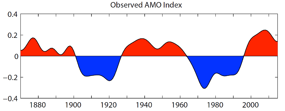
Atlantic Multi-Decadal Oscillation (AMO): The Atlantic Multi-decadal Oscillation is a multidecadal oscillation of sea surface temperatures in the north Atlantic Ocean with an estimated period between 60 and 80 years. The AMO index is determined by removing the long-term trend from the time series and applying smoothing techniques to the inter-annual variability.
The warm phase of the AMO has typically been associated with more active hurricane years in the Atlantic basin and heavier than normal rainfall in the Sahel region of West African, whereas the dry phase has typically been associated with the opposite (drought in the Sahel and suppressed hurricane activity in the Atlantic).
source: https://climatedataguide.ucar.edu/climate-data/atlantic-multi-decadal-oscillation-amo
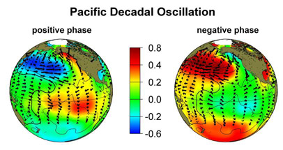
Pacific Decadal Oscillation (PDO): The Pacific Decadal Oscillation is a shorter term (20-30 year) fluctuation in the Pacific Ocean. The sea surface temperature patterns in the tropics for the positive and negative phases are similar to those for El Nino and La Nina, but there are important mid-high latitude teleconnections. In the positive phase of the PDO, warm SST anomalies extend up the US and Canadian coasts up to Alaska, while the central and western north Pacific are cold. The positive PDO tends to bring enhanced precipitation to western North America and suppressed precipitation to the central Pacific and Asia. In the negative phase, the waters up the NW coast of north America are cool, but the waters in the north central and northwest Pacific are warm and Asia is wetter.
source: https://sealevel.jpl.nasa.gov/data/el-nino-la-nina-watch-and-pdo/pacific-decadal-oscillation-pdo/
Long-term Climate Change: Paleoclimate
On still longer time scales, there is clear evidence in the Earth’s history of significant climate changes. This evidence has been gathered from multiple geological and chemical sources: the placement and dating of fossils, the location of glacial striations on rock, evidence of large changes in paleological sea levels, tree ring and coral growth records and the careful measurement of the concentrations specific chemical isotopes (particularly oxygen 18) in glacial ice and in marine and lake sediments that are known to be clear climate indicators.
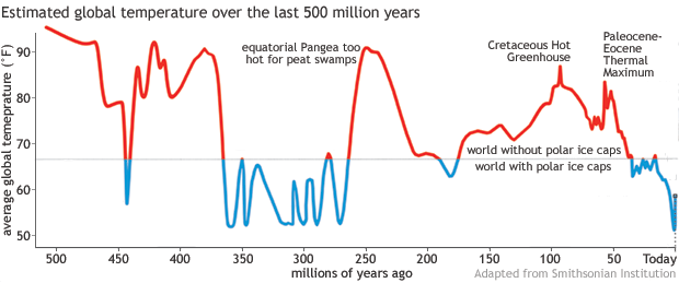
While the very early Earth (first few billion years) was very hot, there is evidence of glaciation in the Neoproterozoic era between 600 and 800 million years ago. Shortly thereafter, there was a significant rise in global mean temperature which led to the Cambrian era’s explosion of life and evolution. The time series of estimated global mean temperature over the last 500 million years is shown below. As is clearly visible, for much of Earth’s history, the global mean temperature was warmer than now (throughout the age of the dinosaurs from 220 to 65 million years ago) and even in the early Cenozoic around 55 million years ago. Furthermore, from the figure below, at a global mean temperature above about 67 F, polar ice caps tend to disappear. The very recent geologic past (last million years or so) have been marked by periods of expanding and contracting glaciation. We also know from paleological evidence that many of the major climate changes in the past have been accompanied by mass extinctions.
Our current global mean temperature is about 59-60F and between Antarctica and Greenland there is approximately 30 million cubic km of glacial ice. If all of that were to melt, it would raise the global mean sea level by almost 100 meters.
source: https://www.climate.gov/news-features/climate-qa/whats-hottest-earths-ever-been
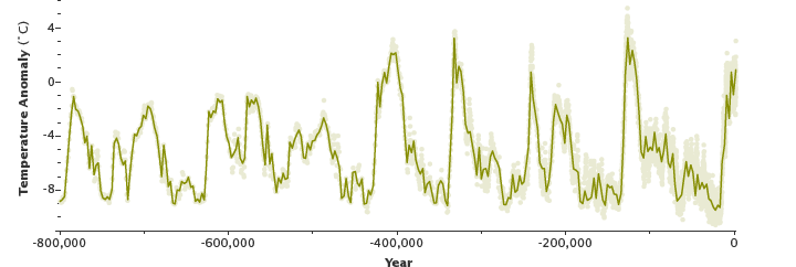
In the last million years or so, there has been a repeated cycle of glacial periods and interglacial periods (during what is known as the Pleistocene period). These are thought to be primarily driven by subtle changes in the Earth’s orbital parameters, which can self-amplify into patterns of growing or shrinking ice caps in the Arctic. This forcing is known as the so called Milankovitch forcing after the Serbian astronomer who proposed the theory. It’s also noticeable from the graphic below that the transition to warm interglacial periods is typically more abrupt than the slower cooling into a period of glaciation.
Ice-core reconstructed temperature anomaly over the last roughly 800 thousand years. Source: National Snow and Ice Data Center
For more information, consult https://earthobservatory.nasa.gov/features/GlobalWarming/page3.php
Anthropogenic Climate Change
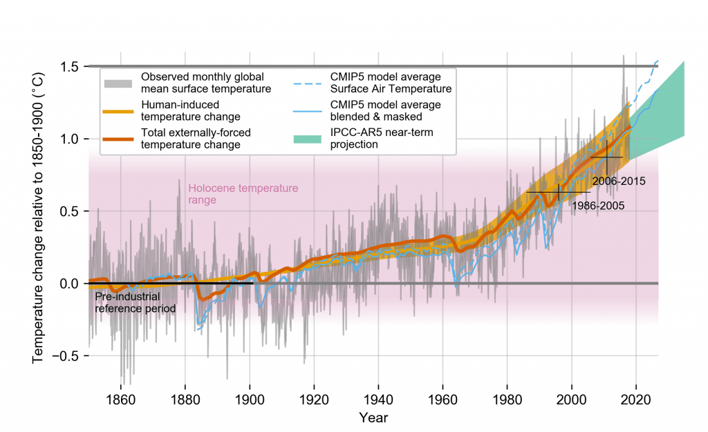
In the present moment and over the last roughly 150 to 200 years, we are, of course, most deeply concerned about the impact of anthropogenic climate change. On the basis of the instrumental record from the period of the industrial revolution to the present, we know that the global mean temperature looks like the graph below.
Source: IPCC special 1.5C report, WGI
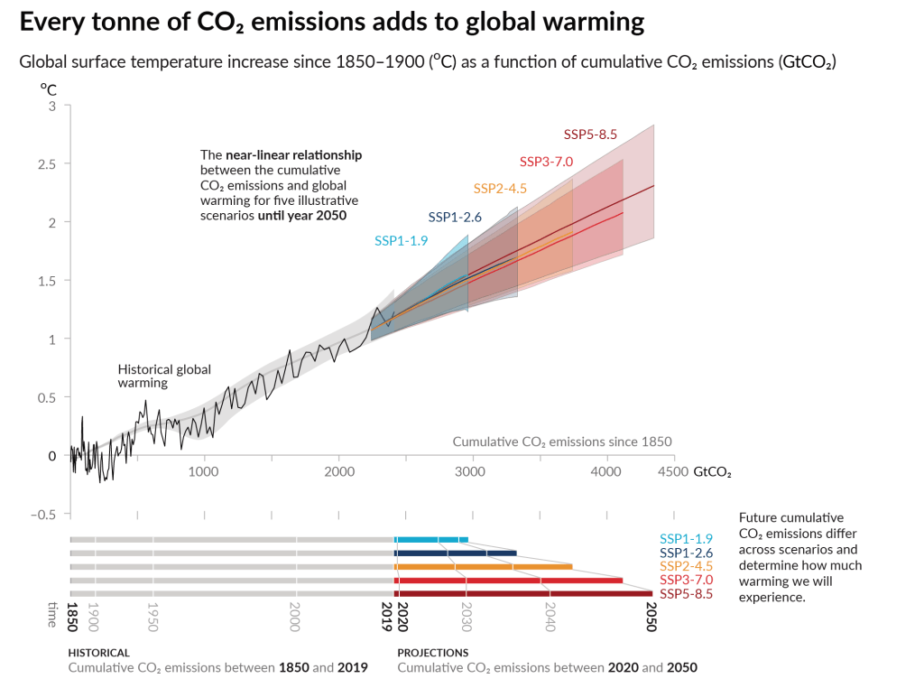
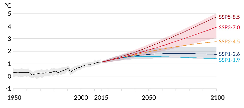
The conclusions of each successive Intergovernmental Panel on Climate Change (IPCC) report have grown increasingly strident and the observational evidence of climate change has grown ever more clear. One of the key tools the IPCC enterprise uses to understand the potential future are a wide series of modeling experiments carried out by the various global climate models (GCMs) using agreed upon emission scenarios. In 2021’s AR6 report, the IPCC developed a new framework for emission scenarios called the shared socioeconomic pathways or SSPs. These scenarios imagine different pathways of economic development, energy use, coordination, etc., to arrive at an understanding of how much carbon might be emitted on what time scale over the balance of the 21st century. This atmospheric forcing is then integrated into the climate models to seek to understand the temperature and other climate related implications. The graphic below frames the
source: IPCC AR6 report, WGI
The projected global mean temperature effects of these SSPs are shown here
source: IPCC AR6 report, WGI
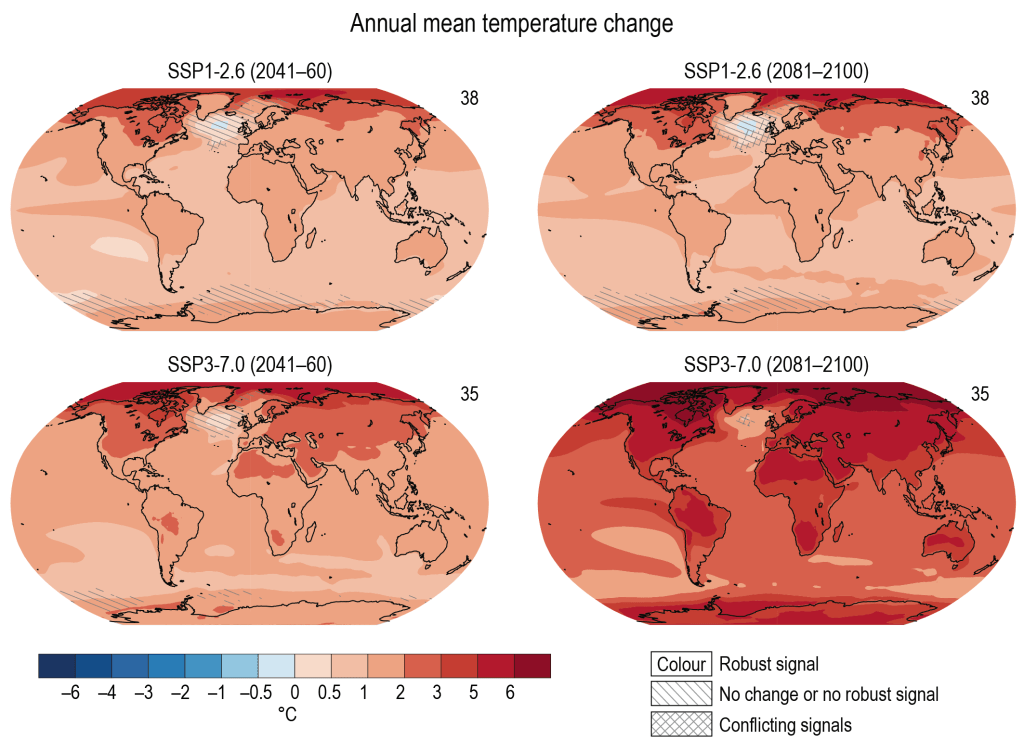
The projected spatial distribution of warming (relative to pre-Industrial levels) for two scenarios and two time horizons is shown in the maps below.
source: IPCC AR6 report, WGI
There are, of course, many other robust conclusions that the IPCC reaches beyond change in the mean temperature, but many of those effects are discussed conceptually on other parts of this website.
