As mentioned in the climate science explained section, anthropogenic climate change generally brings about a significant and disproportionate increase in the frequency of extreme events.
The script below calculates the probability of exceeding a high threshold and not exceeding a low threshold for both an initial (unperturbed state) and for a state under climate change, with a given change in the mean and standard deviation. This code assumes that the variable in question has a normal distribution. Consequently, the equations for the probabilities of exceedance of the high threshold and non-exceedance of the low threshold are shown below.
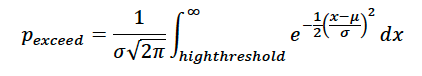

where e is the natural number 2.718, pi is 3.1415, sigma is the standard deviation, mu is the mean and x is the variable in question. Note that if this normal assumption is not valid, the calculation would have to be adjusted to reflect the distribution of the data.
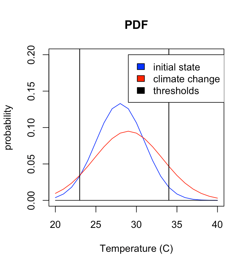
The example given below is for temperature in degrees C with an initial distribution with a mean of 28C and a standard deviation of 3C. The “climate change” scenario increases the mean temperature by 1C and the standard deviation by 40%. The blue curve is the pdf for the initial state and the red curve is the pdf for the climate change state. The threshold values of 34C and 23C are shown as vertical lines. Note that in the warmer climate, there is a considerably higher likelihood of exceeding the warm threshold (area under red curve to the right of 34C). But in the warmer climate with the greater climate variability, there is also somewhat of an increase in the likelihood of the temperature falling below the 23C threshold because of the variability effect.
In addition to calculating the probability of exceeding the high threshold or falling short of the low threshold in the initial and climate change states, the code below also calculates the probability ratio of the climate change/initial state and the so-called “fraction of attributable risk” or FAR. The FAR is bounded by 0 and 1 and is the (probability of the event happening under climate change – the probability of the event happening under the initial conditions)/probability of the event happening under climate change. For really extreme events, the FAR may exceed 0.9 or 0.95 (or 90 or 95% in percentage terms) and the likelihood of the extreme event may be many times greater with climate change than without it. These types of attribution studies and diagnostics have been calculated for some of the major recent extreme events around the world (heat waves in Texas in the early 2010s, and in the Pacific Northwest in 2021) and for some of the most extreme events, the probability that the event would have occurred without climate change is vanishingly small.
R script
#This script calculates the probability of exceeding or not exceeding a given
#threshold in an initial case with specified mean, stdev and skew and in a
#changed case of a specified change in mean, stdev and skew.

thrhigh = 34
thrlow = 23

inimean = 28
inistd = 3

f <- function(x) {exp(-0.5*((x-inimean)/inistd)^2)/(inistd*sqrt(2*pi))}
POEhighinit <- integrate(f, lower = thrhigh, upper = Inf)
print(paste('POEhighinit',POEhighinit$value))
PNElowinit <- integrate(f, lower = -Inf, upper = thrlow)
print(paste('PNElowinit',PNElowinit$value))

dmean = 1
dstd = 1.4
newmean = inimean+dmean
print(paste('newmean',newmean))
newstd = inistd*dstd
print(paste('newstd',newstd))

g <- function(x) {exp(-0.5*((x-newmean)/newstd)^2)/(newstd*sqrt(2*pi))}
POEhighnew <- integrate(g, lower = thrhigh, upper = Inf)
print(paste('POEhighnew',POEhighnew$value))
PNElownew <- integrate(g, lower = -Inf, upper = thrlow)
print(paste('PNElownew',PNElownew$value))

highrat <- POEhighnew$value/POEhighinit$value
lowrat <- PNElownew$value/PNElowinit$value
print(paste('highrat',highrat))
print(paste('lowrat',lowrat))

FARhigh = (POEhighnew$value-POEhighinit$value)/POEhighnew$value
FARlow = (PNElownew$value-PNElowinit$value)/PNElownew$value
print(paste('FARhigh',FARhigh))
print(paste('FARlow',FARlow))

x <- c(20, 21, 22, 22.99, 23, 23.01, 24, 25, 26, 27, 28, 29, 30, 31, 32, 33, 33.99, 34, 34.01, 35, 36, 37, 38, 39, 40)
h <- c(0, 0, 0, 0, 1, 0, 0, 0, 0, 0, 0, 0, 0, 0, 0, 0, 0, 1, 0, 0, 0, 0, 0, 0, 0)
plot(x, f(x), type="l", col="blue", pch="o", lty=1, ylim=c(0,0.2), main = "PDF", xlab = "Temperature (C)", ylab = "probability")
lines(x, g(x), col="red")
lines(x, h, col="black")
legend(29, 0.2, legend=c("initial state", "climate change","thresholds"), fill = c("blue","red","black"))
Python script
#This script calculates the probability of exceeding or not exceeding a given
#threshold in an initial case with specified mean, stdev and skew and in a
#changed case of a specified change in mean, stdev and skew.
import math
import matplotlib.pyplot as plt
import scipy
import scipy.integrate as integrate
from scipy.integrate import quad
import numpy as np

thrhigh = 34
thrlow = 23

inimean = 28
inistd = 3

def integrand(x, inimean, inistd):
    return math.e**(-0.5*((x-inimean)/inistd)**2)/(inistd*math.sqrt(2*math.pi))

POEhighinit = quad(integrand, thrhigh, math.inf, args=(inimean,inistd))
print('POEhighinit',POEhighinit)
PNElowinit = quad(integrand, -math.inf, thrlow, args=(inimean,inistd))
print('PNElowinit',PNElowinit)
dmean = 1
dstd = 1.4
newmean = inimean+dmean
print('newmean',newmean)
newstd = inistd*dstd
print('newstd',newstd)
def integrand(x, newmean, newstd):
    return math.e**(-0.5*((x-newmean)/newstd)**2)/(newstd*math.sqrt(2*math.pi))

POEhighnew = quad(integrand, thrhigh, math.inf, args=(newmean,newstd))
print('POEhighnew',POEhighnew)
PNElownew = quad(integrand, -math.inf, thrlow, args=(newmean,newstd))
print('PNElownew',PNElownew)
highrat = float(POEhighnew[0])/float(POEhighinit[0])
lowrat = float(PNElownew[0])/float(PNElowinit[0])
print('highrat',highrat)
print('lowrat',lowrat)

FARhigh = 1-1/highrat
FARlow = 1-1/lowrat
print('FARhigh',FARhigh)
print('FARlow',FARlow)
x = np.transpose(np.array([20, 21, 22, 23, 23, 23, 24, 25, 26, 27, 28, 29, 30, 31, 32, 33, 34, 34, 34, 35, 36, 37, 38, 39, 40]))
thresholds = np.transpose(np.array([0, 0, 0, 0, 0.2, 0, 0, 0, 0, 0, 0, 0, 0, 0, 0, 0, 0, 0.2, 0, 0, 0, 0, 0, 0, 0]))
f = math.e**(-0.5*((x-inimean)/inistd)**2)/(inistd*math.sqrt(2*math.pi))
g = math.e**(-0.5*((x-newmean)/newstd)**2)/(newstd*math.sqrt(2*math.pi))
plt.title('PDFs')
plt.xlabel('Temperature deg C')
plt.ylabel('probability')
plt.plot(x, f, label = "initial climate")
plt.plot(x, g, label = "altered climate")
plt.plot(x, thresholds, label = "thresholds")
plt.legend()
plt.show()
Matlab script
%This script calculates the probability of exceeding or not exceeding a given
%threshold in an initial case with specified mean, stdev and skew and in a
%changed case of a specified change in mean, stdev and skew.

thrhigh = 34;
thrlow = 23;

inimean = 28;
inistd = 3;

X = [thrhigh Inf];
Y = [-Inf thrlow];

POEhighinit = 0.5*(1+erf((X(1,2)-inimean)/(inistd*sqrt(2))))-0.5*(1+erf((X(1,1)-inimean)/(inistd*sqrt(2))))

PNElowinit = 0.5*(1+erf((Y(1,2)-inimean)/(inistd*sqrt(2))))-0.5*(1+erf((Y(1,1)-inimean)/(inistd*sqrt(2))))

dmean = 1;
dstd = 1.4;
newmean = inimean+dmean
newstd = inistd*dstd

POEhighnew = 0.5*(1+erf((X(1,2)-newmean)/(newstd*sqrt(2))))-0.5*(1+erf((X(1,1)-newmean)/(newstd*sqrt(2))))

PNElownew = 0.5*(1+erf((Y(1,2)-newmean)/(newstd*sqrt(2))))-0.5*(1+erf((Y(1,1)-newmean)/(newstd*sqrt(2))))

highrat = POEhighnew/POEhighinit
lowrat = PNElownew/PNElowinit


FARhigh = 1-1/highrat
FARlow = 1-1/lowrat

x = [20, 21, 22, 23, 23, 23, 24, 25, 26, 27, 28, 29, 30, 31, 32, 33, 34, 34, 34, 35, 36, 37, 38, 39, 40];
thresholds = [0, 0, 0, 0, 0.2, 0, 0, 0, 0, 0, 0, 0, 0, 0, 0, 0, 0, 0.2, 0, 0, 0, 0, 0, 0, 0];
f = exp(-0.5*((x-inimean)/inistd).^2)/(inistd*(2*pi).^0.5);
g = exp(-0.5*((x-newmean)/newstd).^2)/(newstd*(2*pi).^0.5);
plot(x,f,x,g,x,thresholds)
title('PDFs')
xlabel('Temperature deg C')
ylabel('probability')
legend('initial climate','altered climate','thresholds')
