An important question for applied climate science is to understand how frequently an extreme event of a particular magnitude is likely to happen in a given time horizon. While there are many complex dynamical feedbacks in the climate system that can help inform the answer to this question (particularly if the time horizon is relatively short), we can also approach this question statistically by using Monte Carlo methods. With this code, the user can design m iterations of length n with a specified mean and standard deviation and then consider the role of imposed trends in the mean and standard deviation on the frequency of extreme events. As with the other extremes page, the assumption here is that the geophysical variable in question has a Gaussian/normal distribution.
In addition to the effects of changes in the mean and standard deviation, another key factor in understanding climate variability is the role of decadal variability. Decadal variability can be modeled in a crude statistical way by using temporal autoregression, with stronger temporal autoregression values basically indicating a stronger (and longer period) mode of multi-decadal variability.
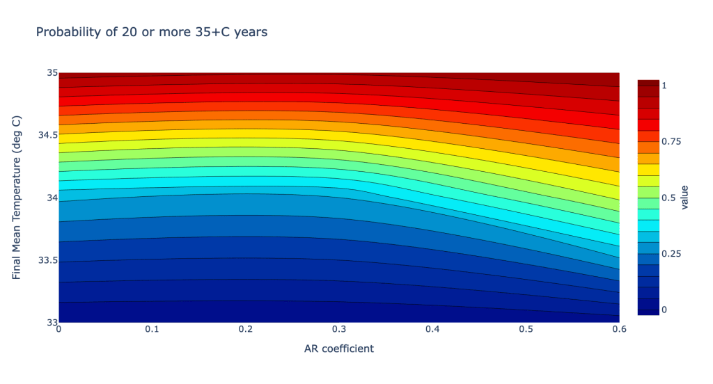
In addition to understanding how frequently a threshold is crossed in absolute terms, it is also important (particularly for insurance companies and other financial institutions with financial obligations contingent on damage) to understand the likelihood of a string of extreme events in a given time window. In the code below, 100 simulations are run of 101 years with an initial temperature distribution with mean 31C and standard deviation 2C. Three scenarios are envisioned regarding trends in the mean and standard deviation. Trend 1 has a final mean temperature of 33C, trend 2 has a final mean temperature of 34 C and trend 3 has a final mean temperature of 35C. Scenario 1 has a standard deviation that grows from 2C to 2.4C over the 101 years. Scenario 2 has a standard deviation that grows from 2C to 2.5C over the 101 years. Scenario 3 has a standard deviation that grows from 2C to 2.6C over the 101 years. Additionally, three MDV/autoregressive scenarios are constructed with the lag 1 year AR coefficient being 0, 0.3 and 0.6 respectively with the higher AR coefficients indicating stronger persistence in the climate system.
In the graphic below, the probability of 20 more years (out of 101) with mean temperatures above 35C is plotted in the colorscale as a function of the final mean temperature (and associated change in variance) (Y axis) and the autoregression coefficient (X axis).
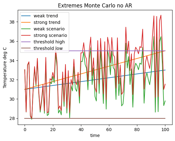
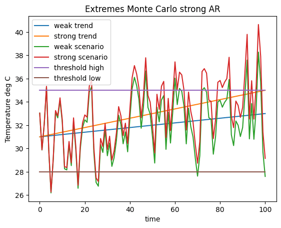
The line plots below show example simulations from the Monte Carlo analysis, the high temperature threshold (35C), a low temperature threshold (28C) and the trendlines for strong and weak warming (to 35 and 33 C respectively). The top graphic is for AR1 = 0. The bottom graphic is for AR1 = 0.6.
R script
#This script conducts a Monte Carlo simulation of length n, with m experiments
#to determine the probability of crossing thresholds.

#length of data (n) and number of experiment (m)
n = 41
m = 20

#The initial mean, stdev threshold and autoregressive coefficients in raw units
meanini = 31
stdini = 2
meanfin = 33
stdfin = 2.4
threshigh = 34
threslow = 28
AR = 0.2

#redefinition of means, standard deviations, trends and thresholds in
#standardized units
meaniniz = meanini-meanini
stdiniz = stdini/stdini

#high and low thresholds

thrhighz = (threshigh-meanini)/stdini
thrlowz = (threslow-meanini)/stdini

#initial mean and standard deviation and interval size of linear trend in mean
#and std

meanendz = (meanfin-meanini)/stdini
meanitvlz = meanendz/(n-1)

stdendz = stdfin/stdini
stditvlz = (stdendz-stdiniz)/(n-1)

#definitions of trends in mean and stdev
trendz = seq(meaniniz,meanendz,meanitvlz)
stdtrendz = seq(stdiniz,stdendz,stditvlz)
print(trendz)
print(stdtrendz)

#A is defined random matrix of probabilities. B is defined matrix of z scores of
#A. C multiplies the z score matrix by the stdtrend point by point. D adds the
#mean trend to the modulated z scores.
A <- matrix(runif(m*n),nrow=n)
print(A)
B = qnorm(A, mean = 0, sd = 1, lower.tail = TRUE, log.p = FALSE)
print(B)
C <- matrix(NA,n,m)
for (i in 1:1) {C[i,] = B[i,]}
for (i in 2:n) {C[i,] = AR*B[i-1,]+(1-AR)*B[i,]}
print(C)
D = C*stdtrendz
print(D)
E = D+trendz
print(E)

#E is the number of high threshold exceedances and probability. G is number of
#low threshold non-exceedances and probability
G = sum(E>=thrhighz)
print(G)
print(paste('probability of exceeding high threshold',G/(n*m)))
H = sum(E<=thrlowz)
print(H)
print(paste('probability of not exceeding low threshold',H/(n*m)))

x = seq(1,n,1)
print(x)
thresholdhigh = rep(c(threshigh), each = n)
thresholdlow = rep(c(threslow), each = n)
plot(x, (trendz)*stdini+meanini, type="l", col="blue", lty=1, ylim=c(10,40), main = "Extremes Monte Carlo", xlab = "time", ylab = "Temperature deg C")
lines(x, (E[,1])*stdini+meanini, col="red")
lines(x, (E[,2])*stdini+meanini, col = "green")
lines(x, thresholdhigh, label = "black")
lines(x, thresholdlow, label = "grey")
legend(0, 25, legend=c("mean trend", "climate scenario 1","climate scenario 2", "high threshold", "low threshold"), fill = c("blue","red", "green", "black","grey"))
Python script
#This script displays the probability of crossing an extreme threshold a specified
#number of times in a given time window on the basis of Monte Carlo simulation with
#imposed trends in mean, standard deviation and a range of autoregression coefficients.
#This script conducts a Monte Carlo simulation of length n, with m experiments
#to determine the probability of crossing thresholds.

import pandas as pd
import numpy as np
import scipy.stats as stats
import matplotlib.pyplot as plt
import plotly.graph_objects as go
import plotly.express as px


#length of data (n) and number of experiment (m)
n = 101
m = 100

#The initial mean, stdev, final mean and standard deviations for three scenarios, low and high thresholds and autoregressive coefficients in raw units
meanini = 31
stdini = 2
meanfin1 = 33
stdfin1 = 2.4
meanfin2 = 34
stdfin2 = 2.5
meanfin3 = 35
stdfin3 = 2.6
threshigh = 35
threslow = 28
freqthresh = 20
AR1 = 0.0
AR2 = 0.3
AR3 = 0.6

#redefinition of means, standard deviations, trends and thresholds in standardized units
meaniniz = meanini-meanini
stdiniz = stdini/stdini

#high and low thresholds in standardized units

thrhighz = (threshigh-meanini)/stdini
thrlowz = (threslow-meanini)/stdini

#final mean and standard deviation and interval size of linear trend in mean and std for three scenarios

meanendz1 = (meanfin1-meanini)/stdini
meanitvlz1 = meanendz1/(n-1)

stdendz1 = stdfin1/stdini
stditvlz1 = (stdendz1-stdiniz)/(n-1)

meanendz2 = (meanfin2-meanini)/stdini
meanitvlz2 = meanendz2/(n-1)

stdendz2 = stdfin2/stdini
stditvlz2 = (stdendz2-stdiniz)/(n-1)

meanendz3 = (meanfin3-meanini)/stdini
meanitvlz3 = meanendz3/(n-1)

stdendz3 = stdfin3/stdini
stditvlz3 = (stdendz3-stdiniz)/(n-1)

#definitions of trends in mean and stdev for three scenarios
trendz1 = np.array([np.arange(meaniniz,meanendz1+0.0000000001,meanitvlz1),]*m)
stdtrendz1 = np.array([np.arange(stdiniz,stdendz1+0.000000001,stditvlz1),]*m)
trendz2 = np.array([np.arange(meaniniz,meanendz2+0.00000000001,meanitvlz2),]*m)
stdtrendz2 = np.array([np.arange(stdiniz,stdendz2+0.00000000001,stditvlz2),]*m)
trendz3 = np.array([np.arange(meaniniz,meanendz3+0.00000000001,meanitvlz3),]*m)
stdtrendz3 = np.array([np.arange(stdiniz,stdendz3+0.00000000001,stditvlz3),]*m)

#A is defined random matrix of probabilities. B is defined matrix of z scores of A.
A = np.random.rand(n,m)
print(A)
B = stats.zscore(A)
print(B)

#C modifies B by adding the autoregressive coefficient to simulate multidecadal variability.
#C1 is for the low AR case. C2 is for the medium AR case and C3 is for the high AR case.
#The mean of C should be close to zero. The addition of strong autocorrelation slightly expands the standard deviation.

C1 = np.zeros((n,m))
C1[0,] = B[0,]
for i in range(1,n):
    C1[i,] = AR1*B[i-1,]+B[i,]
print(C1)
C2 = np.zeros((n,m))
C2[0,] = B[0,]
for i in range(1,n):
    C2[i,] = AR2*B[i-1,]+B[i,]
print(C2)
C3 = np.zeros((n,m))
C3[0,] = B[0,]
for i in range(1,n):
    C3[i,] = AR3*B[i-1,]+B[i,]
print(C3)

#The E matrices multiply the C1 matrix by the appropriate trend in standard deviation element by element.
#The subscript 11 means weak autocorrelation, weak trend, 13 means weak autocorrelation, strong trend, etc..
#I.e. if there is a trend towards an increasing standard deviation, the latest time slices of the E matrix
#will have a larger standard deviation than the earlier time slices.
#The F matrices then add the E matrices with the appropriate trend in the mean.

E11 = np.multiply(C1,np.transpose(stdtrendz1))
F11 = np.add(E11,np.transpose(trendz1))

E12 = np.multiply(C1,np.transpose(stdtrendz2))
F12 = np.add(E12,np.transpose(trendz2))

E13 = np.multiply(C1,np.transpose(stdtrendz3))
F13 = np.add(E13,np.transpose(trendz3))

E21 = np.multiply(C2,np.transpose(stdtrendz1))
F21 = np.add(E21,np.transpose(trendz1))

E22 = np.multiply(C2,np.transpose(stdtrendz2))
F22 = np.add(E22,np.transpose(trendz2))

E23 = np.multiply(C2,np.transpose(stdtrendz3))
F23 = np.add(E23,np.transpose(trendz3))

E31 = np.multiply(C3,np.transpose(stdtrendz1))
F31 = np.add(E31,np.transpose(trendz1))

E32 = np.multiply(C3,np.transpose(stdtrendz2))
F32 = np.add(E32,np.transpose(trendz2))

E33 = np.multiply(C3,np.transpose(stdtrendz3))
F33 = np.add(E33,np.transpose(trendz3))


#G is the number of high threshold exceedances and probability. H is number of
#low threshold non-exceedances and probability
G11 = sum(F11>=thrhighz)
print('G11',G11)
H11 = sum(F11<=thrlowz)
print('H11',H11)
G12 = sum(F12>=thrhighz)
print('G12',G12)
H12 = sum(F12<=thrlowz)
print('H12',H12)
G13 = sum(F13>=thrhighz)
print('G13',G13)
H13 = sum(F13<=thrlowz)
print('H13',H13)
G21 = sum(F21>=thrhighz)
print('G21',G21)
H21 = sum(F21<=thrlowz)
print('H21',H21)
G22 = sum(F22>=thrhighz)
print('G22',G22)
H22 = sum(F22<=thrlowz)
print('H22',H22)
G23 = sum(F23>=thrhighz)
print('G23',G23)
H23 = sum(F23<=thrlowz)
print('H23',H23)
G31 = sum(F31>=thrhighz)
print('G31',G31)
H31 = sum(F31<=thrlowz)
print('H31',H31)
G32 = sum(F32>=thrhighz)
print('G32',G32)
H32 = sum(F32<=thrlowz)
print('H32',H32)
G33 = sum(F33>=thrhighz)
print('G33',G33)
H33 = sum(F33<=thrlowz)
print('H33',H33)

#Lowercase g entries show the frequency with which the m simulations exceeded the high threshold
#(in this case 35 C) by at least the frequency threshold (in this case at least 20 times) in the
#time series length n (in this case 101 years).
g11 = sum(G11>=freqthresh)/m
g12 = sum(G12>=freqthresh)/m
g13 = sum(G13>=freqthresh)/m
g21 = sum(G21>=freqthresh)/m
g22 = sum(G22>=freqthresh)/m
g23 = sum(G23>=freqthresh)/m
g31 = sum(G31>=freqthresh)/m
g32 = sum(G32>=freqthresh)/m
g33 = sum(G33>=freqthresh)/m

print('G', g11, g12, g13, g21, g22, g23, g31, g32, g33)

#This section of code plots the lowercase g coefficients in a matrix with a smooth interpolation
#contour plot to indicate the probability of exceeding the high threshold at least the frequency
#threshold number of times as a function of change in mean (and standard deviation) and AR coefficient.
fig = go.Figure(data =
    go.Contour(
        z=[[g11, g21, g31],
           [g12, g22, g32],
           [g13, g23, g33]],
        x=[AR1, AR2, AR3],
        y=[meanfin1, meanfin2, meanfin3],
       colorscale = 'Jet',
       contours=dict(
           start=0,
           end=1,
           size=0.05,

       ),
        colorbar=dict(
            title='value', # title here
            titleside='right',
            titlefont=dict(
                size=14,
                family='Arial, sans-serif')),

        ))
fig.update_layout(title='Probability of 20 or more 35+C years')
fig['layout']['yaxis'].update(title='Final Mean Temperature (deg C)')
fig['layout']['xaxis'].update(title='AR coefficient')


fig.show()

#This code plots the high and low thresholds, the strong and weak warming trend lines and a sample scenario
#from each strong and weak warming trend scenarios using 0 AR.


x = list(range(0,n,1))
thresholdhigh = np.transpose(np.full((1,n),threshigh))
thresholdlow = np.transpose(np.full((1,n),threslow))
plt.title('Extremes Monte Carlo no AR')
plt.xlabel('time')
plt.ylabel('Temperature deg C')
plt.plot(x, np.transpose(trendz1[0,])*stdini+meanini, label = "weak trend")
plt.plot(x, np.transpose(trendz3[0,])*stdini+meanini, label = "strong trend")
plt.plot(x, (F11[:,0])*stdini+meanini, label = "weak scenario")
plt.plot(x, (F13[:,0])*stdini+meanini, label = "strong scenario")
plt.plot(x, thresholdhigh, label = "threshold high")
plt.plot(x, thresholdlow, label = "threshold low")
plt.legend()
plt.show()

#This code plots the high and low thresholds, the strong and weak warming trend lines and a sample scenario
#from each strong and weak warming trend scenarios using the strong AR (in this case 0.6).

x = list(range(0,n,1))
thresholdhigh = np.transpose(np.full((1,n),threshigh))
thresholdlow = np.transpose(np.full((1,n),threslow))
plt.title('Extremes Monte Carlo strong AR')
plt.xlabel('time')
plt.ylabel('Temperature deg C')
plt.plot(x, np.transpose(trendz1[0,])*stdini+meanini, label = "weak trend")
plt.plot(x, np.transpose(trendz3[0,])*stdini+meanini, label = "strong trend")
plt.plot(x, (F31[:,0])*stdini+meanini, label = "weak scenario")
plt.plot(x, (F33[:,0])*stdini+meanini, label = "strong scenario")
plt.plot(x, thresholdhigh, label = "threshold high")
plt.plot(x, thresholdlow, label = "threshold low")
plt.legend()
plt.show()
Matlab script
%This program will stochastically simulate extreme events for a range of
%climate change scenarios and multi-decadal variability strengths. The
%default is 1000 simulations, run for 100 years with lag 1 autocorrelations of
% 0, 0.2, 0.4, 0.6, 0.8 and 1. The threshold value can be specified by the user.

n = 41
m = 20

%The initial mean, stdev threshold and autoregressive coefficients in raw units
meanini = 31
stdini = 2
meanfin = 33
stdfin = 2.4
threshigh = 34
threslow = 28
AR = 0.6

%redefinition of means, standard deviations, trends and thresholds in
%standardized units
meaniniz = meanini-meanini
stdiniz = stdini/stdini

%high and low thresholds

thrhighz = (threshigh-meanini)/stdini
thrlowz = (threslow-meanini)/stdini

%initial mean and standard deviation and interval size of linear trend in mean
%and std

meanendz = (meanfin-meanini)/stdini
meanitvlz = meanendz/(n-1)

stdendz = stdfin/stdini
stditvlz = (stdendz-stdiniz)/(n-1)

trendz = meaniniz:meanitvlz:meanendz
stdtrendz = stdiniz:stditvlz:stdendz
trendz'
stdtrendz'
TRENDZ = repmat(trendz',1,m)
STDTRENDZ = repmat(stdtrendz',1,m)
zsc = @(p)-sqrt(2)*erfcinv(p*2)

A = rand(n,m,1)

B = zsc(A)

C = zeros(n,m)

C(1,:) = B(1,:)
for i = 2:n
   C(i,:) = AR*B(i-1,:)+(1-AR)*B(i,:)
end

D = C.*STDTRENDZ
E = D+TRENDZ

%E is the number of high threshold exceedances and probability. G is number of
%low threshold non-exceedances and probability
G = sum(sum(E>=thrhighz))
H = G/(n*m)
J = sum(sum(E<=thrlowz))
K = J/(n*m)
Estar = [[0, 0, 0, 0, 0, 0, 0, 0, 0, 0, 0, 0, 0, 0, 0, 0, 0, 0, 0, 0];E];
trendzstar = [0,trendz];
x = transpose([0:1:n]);
thresholdhigh = threshigh*ones(n+1,1);
thresholdlow = threslow*ones(n+1,1);

plot(x, trendzstar'.*stdini+meanini, x, Estar(:,1).*stdini+meanini, x, Estar(:,2).*stdini+meanini, x, thresholdhigh, x, thresholdlow)
title('Extremes Monte Carlo')
xlabel('time')
ylabel('Temperature deg C')
legend('mean trend','climate scenario 1','climate scenario 2','high threshold','low threshold')
