Weather Prediction Overview: The science of weather and climate prediction is complex. Weather refers to shorter time scales (generally up to about two weeks). As mentioned on the climate variability and prediction page, there has been enormous progress since the mid-20th century in predicting weather (temperature, rainfall, humidity, wind speed and direction, surface air pressure). This is thanks to numerous conceptual advances in understanding, the profound improvements in computational capabilities throughout the computer era and the deployment of a wide range of observational equipment (from meteorological stations to weather balloons and radiosondes, to a wide array of satellite-based observations). Weather prediction is generally approached from a dynamical rather than statistical perspective and the information that is disclosed in weather forecasts tends to be fairly deterministic (when you look at a TV weather forecast you see what the expected high and low temperatures are for several days into the future and on which days precipitation is expected and how much – although many contemporary weather forecasts will estimate the likelihood of rain or snow on a given day).
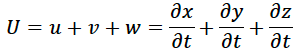
Geophysical Fluids: The governing equations of weather prediction are the complex, nonlinear Navier-Stokes equations – named after the 19th century French and British physicists Claude-Louis Navier and George Stokes who formulated them. Because of their nonlinear nature, they cannot be solved exactly, but with more observational data and more advanced computing power, they can be better constrained. In essence, however, the Navier-Stokes equations are a restatement of Newton’s laws for fluids. There are many formulations of the equations with different assumptions underpinning each and different applications. But here, I will present the most common and most general form for application in climate science. Consider a three dimensional fluid velocity vector U with components u, v and w that represent the component of fluid motion in the x (east/west), y (north/south) and z (vertical) directions.
where the lower case delta represents partial differentiation and t represents time. The mass conservation or “continuity” condition states that mass cannot be created or destroyed and so the local change in mass in a region (and it’s effect on surrounding regions) must be balanced by the horizontal and vertical movement of fluids from nearby locations. In mathematical terms, this is
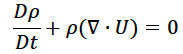
where rho is the density of the fluid. The D/Dt notation is known as the “material derivative” and can be expanded as follows
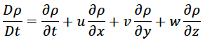
The second term contains an upside down delta symbol, which in mathematical terms is the “gradient operator”. The meaning is given by
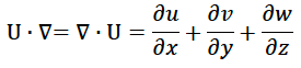
The principle of conservation of momentum (Newton’s second law) can be written as
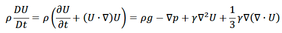
where p is the pressure, g is the gravitational constant, and gamma is the viscosity and other terms are as defined earlier. The gradient2 term is known as the Laplacian operator and is the second derivative of the vector in question. For fluids that do not change density with time, the gradient of the velocity vector is 0 and the last term on the right side of this equation vanishes.
Fluid motions motions in the atmosphere and oceans must satisfy these equations and thermodynamic equations for energy balance and must do so on a rotating planet. This introduces the “Coriolis effect”. For an explanation of this concept, see the video below
Large scale fluid motions in the oceans and atmosphere tend towards a state of quasi-geostrophic balance, wherein the pressure gradient, Coriolis effect and frictional forces approximately balance each other. In global weather and climate models, the Navier-Stokes equations are solved for each gridbox and layer in the horizontal and vertical dimensions and a wide range of forcings are integrated into the model code.
Nonlinearity and Chaos: MIT mathematician and meteorologist Ed Lorenz demonstrated in the early 1960s that with a nonlinear system of differential equations simpler than the Navier-Stokes equations, very small differences in initial conditions (between two experiments) grow over time to the point where, the results diverge completely and are “chaotic”. He postulated therefore that attempts to constrain the outcomes of weather forecasting beyond a certain length of time would be fruitless and further research has found this limitation to be in the range of 10-14 days lead time. His seminal discovery is often referred to as the “butterfly effect” – after the idea that if a butterfly flaps its wings in one region of the world, that small perturbation of air pressure and flow could propagate through the atmosphere and induce a major storm at some other remote location. The analogy is a bit hyperbolic, but captures the essential chaotic/nonlinear nature of weather. Lorenz is regarded as a pioneering scholar in both applied math and meteorology for his contribution to both fields. In Lorenz’s system of equations, while the trajectories of differing initial conditions diverge, they do coalesce around a semi-ordered structure, known as a “Lorenz attractor”.
Dynamical Climate Prediction Overview: As seen above, while the ocean and atmosphere act in a manner consistent with Newton’s laws through the Navier-Stokes equations, because of their non-linear nature, there are practical limitations to prediction of precise outcomes. However, it should be noted that the objective of climate modeling is not to predict precise outcomes (what the temperature or rainfall will be like on some specific date seven years in the future at a specific location). For climate prediction, mathematically, the problem is mostly a boundary value problem rather than an initial value problem. Global climate models still approach climate projection and prediction in a dynamical manner, but the parameters are different.
ENSO prediction: One of the most important features in the coupled climate system is the El Nino-La Nina phenomenon or El Nino/Southern Oscillation (ENSO). This phenomenon is described qualitatively on the climate variability and prediction page. In the early 1900s, mathematician Gilbert Walker observed that famine and drought in India were correlated to the sea level pressure differences between the Pacific island of Tahiti and Darwin, Australia. This pressure difference became known as the Southern Oscillation. In the 1960s, meteorologist Jacob Bjerknes connected the Southern Oscillation pressure differences to anomalies in sea surface temperature patterns in the equatorial Pacific and was able to explain the persistence of the El Nino and La Nina states, but didn’t have a good explanation for the transition between the states. Differences in heating drive differences in sea level pressure, resultant winds and associated patterns of rainfall. In the 1970s, oceanographer Klaus Wyrtki developed a set of subsurface observations that shed light on how the depth of the thermocline changed with ENSO phase. In the 1980s, oceanographer Mark Cane and meteorologist Stephen Zebiak developed the “delayed recharge oscillator model” of the ENSO system and made the first successful prediction of an El Nino event. The governing equations of this system are a set of nonlinear dynamical differential equations described the following papers:
Because the governing equations of this system are non-linear, ENSO’s behavior and period is also chaotic and the length of a cycle from fully developed El Nino to neutral to La Nina, to neutral back to El Nino again may take anywhere from 3-7 years and may exhibit more chaotic behavior.
In the years since the development of the Cane-Zebiak model, many other nuanced observations of ENSO have arisen, characterizing different types and evolutions of ENSO behavior (references to Modoki and other types of ENSO), typical and less typical teleconnection patterns (Ropelewski and Halpert 1987, ) and some additional theoretical advances have been made (Chen and Jin 2022?).
Statistical Climate Prediction: While ENSO may be the dominant signal at the global scale in the tropics, there are other important modes of climate variability in the tropics and at higher latitudes, the effect of the Coriolis force becomes more important. Furthermore, while there is a nonlinear deterministic framework for understanding ENSO dynamics and published literature on “typical” ENSO teleconnections, the actual climatic impacts (rainfall, temperature, humidity, winds) experienced in different regions of the world are never perfectly correlated to ENSO state. It is therefore advantageous to use statistical methods, coupled with observations and climate model output to produce sub-seasonal, seasonal and longer range climate forecasts, in an effort to make probabilistic forecast statements.
At the broadest level, the statistical framework that is typically used is a framework of regression. The general practice of regression involves trying to minimize the sum of the square of the errors between predicted and observed values. The simplest form of regression is ordinary least squares (OLS) regression in which the relationship between the predictor and predictand (variable to be predicted) is assumed to be linear. But other forms of regression include exponential or power law regression, polynomial regression, multiple linear regression (MLR), principal component regression (PCR), logistic and extended logistic regression (ELR) and canonical correlation analysis (CCA). Most of the forecasting work that my colleagues and I have done involves PCR, ELR or CCA. We have generally made use of the Climate Predictability Tool (CPT), developed by IRI senior scientist Simon Mason and the more recent Python implementation, PyCPT. Much of the following content is from a training written by Simon.
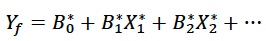
Multiple Linear Regression (MLR): MLR involves making a forecast of a given predictand with multiple predictors that are assumed to have a linear relationship with the predictand. Mathematically, this is expressed as
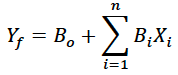
where the Xi are the individual predictors (number = n) and the Bi are the coefficients. MLR can be an effective method if the number of predictors is relatively few and if they are not interrelated. However, if different predictors are highly correlated with each other, one has the problem of collinearity.
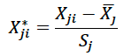
Principal Component Regression (PCR): Principal component regression is optimal for cases with many predictors but few or only one predictand. It addresses the issue of collinearity by creating patterns within the data, called principal components that are perpendicular to each other and then developing a prediction scheme that is based on a linear combination of the principal components. In order to do this, first the predictor data is transformed into standardized form, by subtracting the mean and dividing by the standard deviation
Then a regression equation is made with the transformed X data
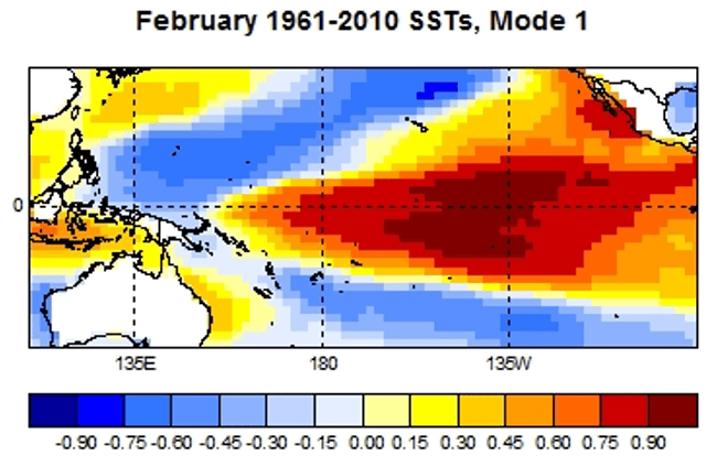
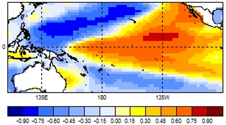
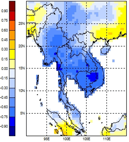
The Bi coefficients are the “weights” for the different predictors in the forecasting scheme. If one is making a forecast using a single type of predictor but a gridded field of data (eg. sea surface temperatures at a 1 degree resolution over a large grid), the Bi “weighting” coefficients turn into a spatial pattern or “mode” in the predictor that is associated with a particular type of anomaly in the predictand.
An example of such a pattern is shown in the diagram below based on a PCR of Pacific sea surface temperatures predicting an index value of rainfall over Thailand.
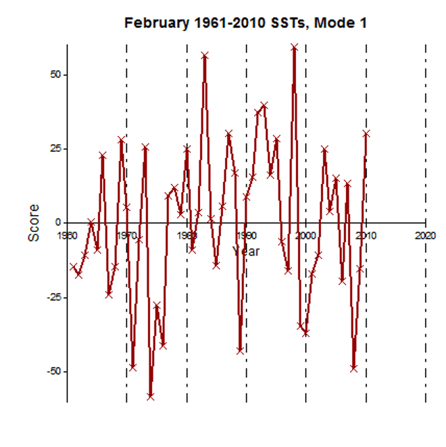
When these weights are multiplied by the actual observations for the given years, a time series of scores is the result as shown below.
Then, the correlation matrix is derived from the adjusted predictors
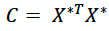
This correlation matrix is a square matrix of length n (where n is the total number of predictors) and has n eigenvalues. The corresponding eigenvector matrix here symbolized as V. The principal component matrix is then given by Z in the following equation.

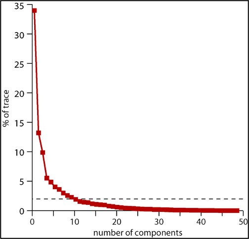
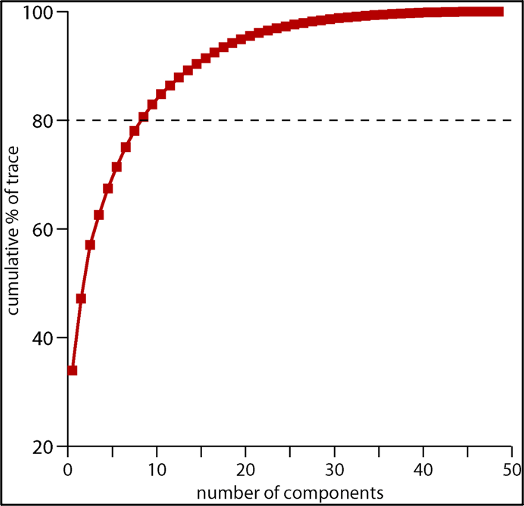
The first principal component always explains the most variance, the second, the second most, etc.. The two diagrams below display for a particular PCR analysis, how much of the variance is explained by each successive mode (upper figure) and the cumulative variance in the predictand explained by all the modes up to that point (lower figure). These “scree plots” can then be used to determine a “stopping rule” regarding how many modes to select.
Canonical Correlation Analysis (CCA): In cases where there is a large number of both predictors and predictands (as with highly resolved gridded data), it is useful to take the logic of principal component regression one step further by using canonical correlation analysis. Rather than establishing “modes” with only the predictor, CCA derives weighting “modes” in both the predictor and predictand fields based on the optimal matching between the multiple predictors and predictands. In addition to these weighting coefficient patterns for the predictor and predictand fields, there are also canonical correlation modes. The leading CCA mode explains the largest share of the variance between the predictor and predictand fields, the second CCA mode, the second most, etc., and each successive mode is perpendicular to the others.
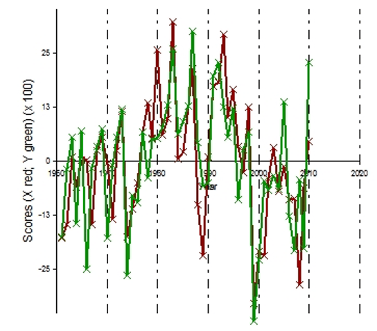
As above, an example is given using Pacific sea surface temperatures to predict rainfall in Thailand (but this time as a gridded field, rather than as an index value).
X mode 1
Y mode 1
scores for observation (green) and predicted (red)
Logistic Regression (Logit) and Extended Logistic Regression (ELR): Logistic regression differs from linear regression and linear regression-based methods like MLR, PCR and CCA in that logistic regression frames observations and predictions in a binary manner and seeks to find a prediction scheme in which the predicted “quantile” matches the observed “quantile” as closely as possible. For this reason, in climate applications and sometimes in other contexts, this approach is also known as quantile regression.
Rather than seeking to minimize the difference in absolute terms (deg C for temperature or mm for rainfall) between observations and predictions, logistic regression seeks to minimize the difference between observations and prediction in “probability space”.
For example, in an academic setting, different students will either pass or fail an exam and they will spend different numbers of hours prepping/studying. Generally, students who study for longer/work harder will tend to have a higher likelihood of passing and/or scoring above any specified threshold, but that relationship may not always hold depending on factors like prior knowledge before the course began, cumulative learning and performance earlier in the semester, pressures from other classes, activities or work responsibilities, issues affecting the students’ personal life, confidence, humility, test taking skill and time management, distractability during studying and during the exam, student intelligence, study strategies, etc.. Hypothetical observations for this scenario are shown below and the blue s-shaped curve shows the regression equation that minimizes the difference in probability space.

In a climate context, a predictor might be something like the distribution of sea surface temperature values in a given region and the predictand might be something like the probability of the rainfall falling in the highest quintile (80th %ile and above). The observed rainfall would be classified as above as being either in that quintile category (1) or not (0). If the sea surface temperature values are generally positively associated with rainfall in a given region (for example higher SSTs in the East Pacific are correlated with heavier rainfall in coastal Peru), the s-shaped logistic curve would hold it’s shape and positive slope and we’d expect that the predicted probability of being in the upper quintile would increase as a function of SST quintile. However, if we are concerned with understanding the lowest quintile in the observations, we would expect that the prediction would most frequently match the observation for the lowest quintile and very few of the high SST scenarios would lead to the rainfall being in the lowest quintile. For intermediate quintiles, this relationship would be more complicated, because we would expect the peak in observed frequency of the quintile of observation to be at the intermediate quintile of the predictor variable(s). But this approach can be applied to each quantile (whether terciles, quartiles, quintiles, deciles or some other division) and predictive coefficients can be derived for each. The math is as follows:
First let us consider a typical regression style equation:
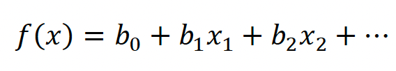
This type of equation can be transformed into an S-shaped curve in probability space through exponentiation and division as follows.
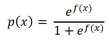
where p(x) is the probability of the event occurring (in the example above the student passing the exam) as a function of the independent variable (time spent studying). The b0, b1, b2, etc. can be considered as the coefficients as in a multiple linear regression example and the different predictors are x1, x2, etc.. With a little algebraic rearrangement, one can then show that
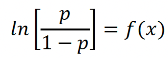
However this formulation has a problem in that it can lead to nonsense/contradictory results – where the cumulative forecast probability of a wet outcome takes a lower probability value than the cumulative forecast probability of a drier outcome. This situation can arise because the regression coefficients for each quantile are determined independently, so the slopes of the regression quantiles can cross each other. This is illustrated in the right half of the diagram below from a paper by Daniel Wilks 2009 in Meteorological Applications. The left side of the same diagram illustrates the outcome of using the “Extended Logistic Regression” method that Wilks formulated and applied to a forecasting context.
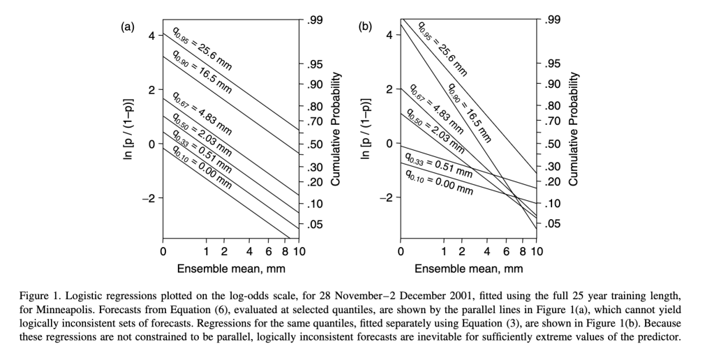
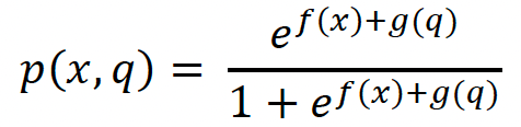
This extended logistic regression approach avoids the spurious scenario of forecast regression lines crossing each other by adding a non-decreasing of quantile g(q) to the regression equation. The mathematical framework is shown below. The probability function is given by
and the extended logistic regression function is related to the natural logarithm of p(q)/(1-p(q)) as follows.
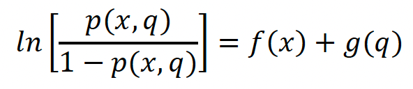
This extended logistic regression formulation can then be used to solve for regression coefficients of all quantiles simultaneously, rather than solving each individually.
Downscaling: For both climate prediction on short time scales and for climate projection on longer time scales, there is often a need for some form of “downscaling”, or translating a signal at a coarse resolution to an output at a much higher resolution. The end user generally wants to know what is likely to happen on his farm or property or in his village (not what is likely to happen in a 1 degree latitude by 1 degree longitude box). Broadly speaking, downscaling can be dynamical (i.e. using a more highly resolved dynamical model nested within a coarser scale model) or statistical (using local scale statistical climate relationships within a region to extrapolate to the local level from coarser scale input).
Dynamical downscaling may offer more precise results with more internally consistent physics, if the model framework is well-developed. But it can suffer from edge effects, model biases and can often be computationally (and financially and temporally) expensive. Statistical downscaling is often cheaper, quicker and less computationally expensive. But the end result may not be as physically consistent and often, in order to do statistical downscaling, there is an assumption that climatic relationships between different regions at a small scale will remain largely the same as the climate changes. This may not be always be accurate as we move to a more significantly altered climate.
