Concentrations for greenhouse gases are often reported in concentrations per unit volume (eg. parts per million by volume). The way to calculate concentration over time is to start with the initial concentration as a mass ratio, figure out the net emissions (emissions-sequestration for each time step) and then add that net emission to each subsequent time step. In the code below, the default numbers refer to the concentration of carbon dioxide with a starting point in 2022 (of 417 ppmv). The molar mass of CO2 (44g) is heavier than that of ordinary atmosphere. The two most dominant chemical species in the troposphere are N2 (almost 80%) and O2 (around 20%). N2 has a molar mass of 28g, while O2 has a molar mass of 32g – so a typical mole of atmosphere weighs on the order of 28.8g. So the 417 ppmv is equivalent to 637 ppmm (parts per million by mass). Given the total mass of the atmosphere (5.15*1015 metric tonnes), this implies that there are currently about 3.3*1012 metric tonnes of carbon dioxide in the atmosphere. Emissions last year were on the order of 37 gigatonnes (of 3.7*1010 tonnes). So, in the absence of any sequestration, this would lead to an increase in concentrations by about 1%/year or about 4 ppmv.
Fortunately, there is some carbon sequestration by the oceans and by biogeochemical processes on land, so the actual observed annual growth in atmospheric concentration has been more like 2 ppmv, rather than 4 ppmv. But there are limitations to this rate of sequestration. The longest standing direct measurement of greenhouse gases is the record of CO2 concentration from the Mauna Loa observatory in Hawaii – sometimes named the “Keeling curve” after Charles Keeling, who began the monitoring program in 1958. While every single year since the record began has had a higher CO2 concentration than the year before, you can clearly see an annual cycle within the long term trend. This annual cycle peaks in April/May, just before northern hemisphere middle and high latitude plant life begins consuming CO2 in great abundance to support photosynthesis. The concentration sinks to it’s lowest value each year in the northern hemisphere autumn at the end of the growing season and then rises through the northern hemisphere winter as the combination of human emissions and global respiration overwhelm the carbon drawdown by photosynthesis in the tropics and southern hemisphere. The photosynthetic activity of the northern hemisphere dominates the global biological signal because there is considerably more land and plant life in the northern hemisphere than in the southern hemisphere.
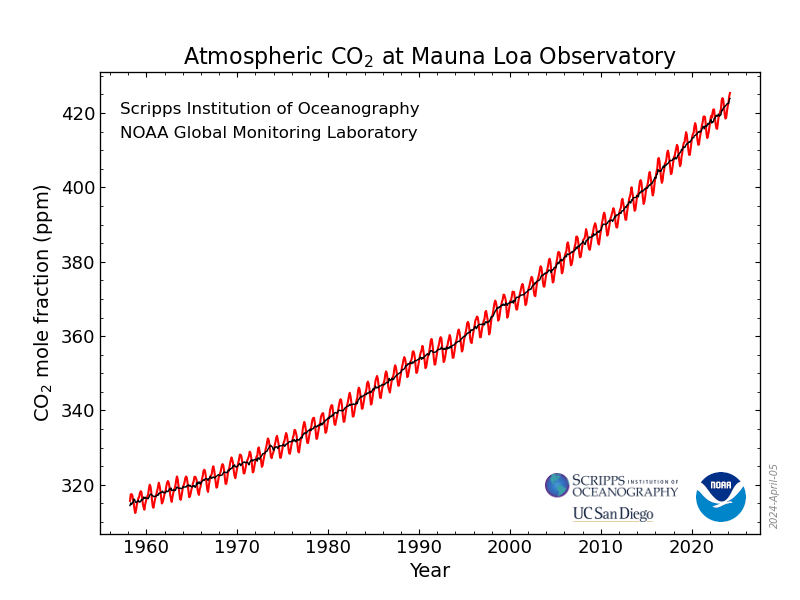
Here is a link to the monitoring project in Mauna Loa: https://gml.noaa.gov/ccgg/trends/
R script
#This script calculates the concentration of GHG (defaults for CO2) from net
#emissions for a number of time steps (n) and a number of scenarios (m).
t <- c(2023, 2024, 2025, 2026, 2027)
n = 5
m = 2
#Mass of the atmosphere and CO2 concentration in 2022 in ppmv.
Matm = 5.148*10^15
conc2022 = 417
#mass ratio and total mass of CO2 in atmosphere (mass ratio is somewhat higher
#than volumetric ratio because CO2 has as higher molar weight (44g) than most
#of the atmosphere. Since the atmosphere is roughly 80% N2 (molar weight 28g)
#and about 20% O2 (molar weight #32 g), the approximate mass of an average
#mole of atmosphere is about 28.8g)
massrat2022 = (conc2022/1000000)*44/28.8
mass2022 = massrat2022*Matm
#emissions and sequestration matrices in gigatonnes arranged  by proceeding
#first through time periods and then through the different scenarios. em and seq
#are real valued emissions and sequestration matrices in tonnes.
emGT <- c(37, 37, 37, 37, 37, 37, 39, 41, 43, 45)
dim(emGT) <- c(n,m)
seqGT <- c(2, 5, 10, 15, 20, 2, 2, 2, 2, 2)
dim(seqGT) <- c(n,m)
em = emGT*10^9
seq = seqGT*10^9
print(em)
print(seq)
#Cumulative emissions (mass) = emissions-sequestration + past net emissions
cumem <- matrix(NA,n,m)
for (i in 1:1) {cumem[i,] = em[i,]-seq[i,]}
for (i in 2:n) {cumem[i,] = em[i,]-seq[i,]+cumem[i-1,]}
print(paste('cumem',cumem))
#convert cumulative emissions to concentration in ppmv+ initial concentration
conc = 1000000*28.8*(mass2022+cumem)/(Matm*44)
print(paste('conc',conc))
plot(t, conc[,1], type="l", col="black", pch="o", lty=1, ylim=c(400,450), main = "Concentration of CO2", xlab = "year", ylab = "ppmv")
lines(t,conc[,2],col="blue")
legend(2023, 410, legend=c("scenario 1", "scenario 2"), fill = c("black","blue"))
Python script
#This script calculates the concentration of GHG (in this case CO2) from net
#emissions for a number of time steps (n) and a number of scenarios (m).
import numpy as np
import matplotlib.pyplot as plt

n = 5
m = 2
#Mass of the atmosphere and CO2 concentration in 2022 in ppmv.
Matm = 5.148*10**15
CO2conc2022 = 417
#mass ratio and total mass of CO2 in atmosphere (mass ratio is somewhat higher
#than volumetric ratio because #CO2 has as higher molar weight (44g) than most
#of the atmosphere. Since the atmosphere is roughly 80% N2 (molar weight 28g)
#and about 20% O2 (molar weight #32 g), the approximate mass of an average
#"mole of atmosphere is about 28.8g)
CO2massrat2022 = (CO2conc2022/1000000)*44/28.8
CO2mass2022 = CO2massrat2022*Matm
#emissions and sequestration matrices in gigatonnes arranged with by proceeding
#first through time periods and then through the different scenarios. em and seq
#are real valued emissions and sequestration matrices in tonnes.
emGT = [[37, 37, 37, 37, 37], [37, 39, 41, 43, 45]]
seqGT = [[2, 5, 10, 15, 20], [2, 2, 2, 2, 2]]
em = np.transpose(np.multiply(emGT,10**9))
seq = np.transpose(np.multiply(seqGT,10**9))
print(em)
print(seq)
#Cumulative emissions (mass) = emissions-sequestration + past net emissions
cumem = np.zeros((n,m))
cumem[0,] = np.subtract(em[0,],seq[0,])
for i in range(1,n):
    cumem[i,] = np.add((np.subtract(em[i,],seq[i,])),cumem[i-1,])
print('cumem',cumem)
#convert cumulative emissions to concentration in ppmv and add starting concentration
conc = 1000000*28.8*(CO2mass2022+cumem)/(Matm*44)
print('conc',conc)

concstar = np.append([[CO2conc2022,CO2conc2022]],conc,axis = 0)
print(concstar)

x = np.transpose(np.array([2022, 2023, 2024, 2025, 2026, 2027]))
plt.title('GHG concentration')
plt.xlabel('year')
plt.ylabel('ppmv')
plt.plot(x, CO2concstar[:,0], label = "scenario 1")
plt.plot(x, CO2concstar[:,1], label = "scenario 2")
plt.legend()
plt.show()
Matlab script
%This script calculates the concentration of GHG (defaults for CO2) from net
%emissions for a number of time steps (n) and a number of scenarios (m).

n = 5;
m = 2;
%Mass of the atmosphere and CO2 concentration in 2022 in ppmv.
Matm = 5.148*10^15;
conc2022 = 417;
%mass ratio and total mass of CO2 in atmosphere (mass ratio is somewhat higher
%than volumetric ratio because CO2 has as higher molar weight (44g) than most
%of the atmosphere. Since the atmosphere is roughly 80% N2 (molar weight 28g)
%and about 20% O2 (molar weight #32 g), the approximate mass of an average
%mole of atmosphere is about 28.8g)
massrat2022 = (conc2022/1000000)*44/28.8;
mass2022 = massrat2022*Matm;
%emissions and sequestration matrices in gigatonnes arranged  by proceeding
%first through time periods and then through the different scenarios. em and seq
%are real valued emissions and sequestration matrices in tonnes with the
%time slices in rows and the scenarios in columns.
emGT = [[37, 37, 37, 37, 37]; [37, 39, 41, 43, 45]];
seqGT = [[2, 5, 10, 15, 20]; [2, 2, 2, 2, 2]];
em = transpose(emGT*10^9)
seq = transpose(seqGT*10^9)
%Cumulative emissions (mass) = emissions-sequestration + past net emissions
for i = 1:n
    netem(i,:) = em(i,:)-seq(i,:);
end
netem
for i = 1:n
    cumem(i,:) = sum(netem(1:i,:),1);
end
cumem
%convert cumulative emissions to concentration in ppmv+ initial concentration
conc = 1000000*28.8*(mass2022+cumem)/(Matm*44)

plot(transpose(t),conc)
title('GHG concentration')
xlabel('year')
ylabel('concentration (ppmv)')
legend('better scenario','worse scenario')
