The amount of global sea level rise is a function of the total melting of land-based glaciers and the increase in temperature of the upper ocean. This code will deal with the sea level rise from those two sources.
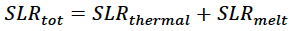
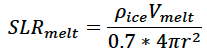
Local gravitational effects, land subsidence or rising (isostatic rebound) will influence local sea level rise to be faster or slower than the global mean. However, the scripts on this page deal with the global sea level rise only as a function of the thermal and melting effects. There are significant uncertainties regarding feedback loops and the potential rate of sea level rise, but the density and volume of glacier ice are fairly well known as is the coefficient of thermal expansion of sea water. The Earth’s surface is about 70% ocean. So to extract the sea level rise from the glacier melt component, one divides the total volume of meltwater, by about 70% the surface area of the Earth (which is 4pir2, where r is the radius of the Earth). Note the volume of meltwater is the volume of melted ice (Vmelt) multiplied by the density ratio of glacier ice/water (rhoice). The total contribution from ice melt is categorized in the manner below.
Note that as sea level gets higher, more land is inundated, so the global area of the ocean slightly increases. But this effect is negligible in the global context, unless sea level rise is quite dramatic.
The contribution of thermal expansion of sea water from warming waters can be characterized as follows
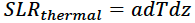
where a is the coefficient of thermal expansion, dT is the change in temperature and dz is the surface layer of the ocean over which there is an appreciable warming. For the example code below, I am considering warming in the upper 100 meters to be relevant/meaningful and warming below that depth to be negligible and inconsequential. The thermal expansion coefficient a = 2.1*10-4mK-1.
The sources of glacial melt are the mountain glaciers, Greenland Ice Sheet, the West Antarctic Ice Sheet, and the East Antarctic Ice Sheet with estimated ice volumes of 170,000 km3, 2.9 million km3, 2.2 million km3 and 27 million km3 respectively. The global approximate density of glacier ice relative to sea water is 0.89. The mean radius of the Earth is 6371 km.
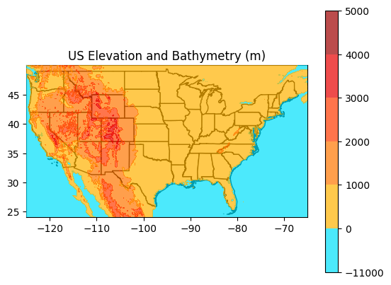
The maps below shows the continental US with different levels of sea level rise using 5 arc minute data from the National Geophysical Data Center (NGDC) (now part of the National Center for Environmental Information (NCEI)). Other higher resolution and higher quality topographic data exist, but this dataset is sufficiently resolved for the purposes here and is projected onto a lat/long grid. Admittedly, while overall topography is the main determinant of inundation, there are local factors at play in inundation – certainly with individual storm surges and even with changes in the mean state.
Scenario 0: No Sea Level Rise, no ocean warming

Scenario 1 (lower impact scenario that has a real chance of occurring this century): 2 degree C rise in surface ocean temperature, 60% loss of all mountain glaciers, 5% loss of the Greenland and West Antarctic Ice Sheets and 1% loss of the East Antarctic Ice Sheet. Total SLR = 1.6 meters (5.3 feet).
While the relationship between the overall global temperature rise and the melt rates of the different reservoirs of ice isn’t fully known this is a plausible scenario by the end of the 21st century. Relatively little land more than 15-20 miles inland would be affected, but many coastal communities and some major coastal cities would be significantly affected in this scenario.
Scenario 2 (very bad scenario very unlikely but not impossible this century): 4 degree C rise in surface ocean temperature, 80% loss of all mountain glaciers, 20% loss of the Greenland and West Antarctic Ice Sheets and 5% loss of the East Antarctic Ice Sheet. Total SLR = 6.35 meters (21 feet).

It’s highly unlikely (but not impossible) that this scenario would be realized by 2100, but it’s possible that the quantity of GHGs put in the atmosphere by 2100 could make this scenario inevitable on a longer time scale. In this scenario, many major coastal cities and communities are lost and there is significant inundation in the coastal areas of a number of coastal states as well as significant losses in Louisiana and Florida. Miami and New Orleans are almost completely underwater. Needless to say – even this scenario, let alone the two more extreme ones presented below constitute a catastrophic impact for the world.
Scenario 3 (catastrophic scenario potentially centuries in the future): 6 degree C rise in surface ocean temperature, 100% loss of all mountain glaciers, 80% loss of the Greenland and West Antarctic Ice Sheets and 20% loss of the East Antarctic Ice Sheet. Total SLR = 25 meters (80 feet).

This scale of sea level rise is almost certainly not possible in the 21st century (the ice melt rate would have to accelerate to the point of producing more than a foot of sea level rise per year…but there is paleoclimatic evidence that the last time global temperatures were as warm as 4 (let alone 6) degrees warmer than the present for an extended period of time, the planet was basically ice free. As you can see, in this scenario there is significant inundation along all major coastlines, including into California’s Central Valley and there is a near complete loss of Florida and Louisiana.
Scenario 4 (worst case scenario several centuries in the future): 8 degree C rise in surface ocean temperature, 100% loss of all permanent ice on the planet. Total SLR = 80 meters (265 feet).

The states of Florida and Louisiana, Delaware and Rhode Island are gone, and there are significant losses to other coastal states across the country – particularly on the Atlantic and Gulf coasts.
R script
# This script calculates the equilibrium sea level change from a given level of
# warming of the upper ocean and melting of Greenland, the West Antarctic Ice
# Sheet and East Antarctica.

dT = 3
dz = 100

# coefficient of thermal expansion
k = 2.1*10^(-4)

#sea level rise from thermal effect alone
SLRt <- k*dT*dz
print(paste('SLRt',SLRt))

#Approximate volumes of the Greenland, West Antarctic and East Antarctic Ice
#Sheets in cubic km.
VMG = 170000
VGreen = 2900000
VWAIS = 2200000
VEAIS = 27000000
# Density of glacier ice relative to sea water
rho = 0.89
#fraction of melt of the Greenland, West Antarctic and East Antarctic Ice Sheets
fMG = c(1,0.7)
fGreen = c(0.1, 0.05)
fWAIS = c(0.1, 0.05)
fEAIS = c(0.02, 0.01)

#total sea level rise (in m) from both thermal expansion and glacier melt
SLRtot <- SLRt+1000*rho*(fMG*VMG+fGreen*VGreen+fWAIS*VWAIS+fEAIS*VEAIS)/(0.7*4*pi*6371*6371)
print(paste('SLRtot',SLRtot))
SLRtotft = 3.281*SLRtot
print(paste('SLRtotft',SLRtotft))
Python script
# This script calculates the equilibrium sea level change from a given level of
# warming of the upper ocean and melting of Greenland, the West Antarctic Ice
# Sheet and East Antarctica.
import math
import numpy as np
# average temperature change of the top 100 m (assuming no appreciable warming
# below).

dT = 2,

dz = 100
# coefficient of thermal expansion
k = 2.1*10**(-4)

#sea level rise from thermal effect alone
SLRt = np.multiply(100*k*dz,dT)
print('SLRt',SLRt)
#Approximate volumes of the Greenland, West Antarctic and East Antarctic Ice
#Sheets in cubic km.
VMG = 170000
VGreen = 2900000
VWAIS = 2200000
VEAIS = 27000000
# Density of glacier ice relative to sea water
rho = 0.89
#fraction of melt of the Greenland, West Antarctic and East Antarctic Ice Sheets
fMG = 0.8
fGreen = 0.03
fWAIS = 0.03
fEAIS = 0.01

#total sea level rise from both thermal expansion and glacier melt
SLRtot = SLRt+1000*rho*(np.multiply(fMG,VMG)+np.multiply(fGreen,VGreen)+np.multiply(fWAIS,VWAIS)+np.multiply(fEAIS,VEAIS))/(0.7*4*math.pi*6371*6371)
print('SLRtot',SLRtot)
SLRtotft = 3.281*SLRtot
print('SLRtotft',SLRtotft)

# Load sample earth political boundaries

worldborders = gpd.read_file("Data/world-administrative-boundaries.shp")
ax = worldborders.clip([-180, -90, 180, 90]).plot(color="white", edgecolor="black")

USstates = gpd.read_file("Data/cb_2018_us_state_500k.shp")
ax = USstates.clip([-76, 38, -73, 42]).plot(color="white", edgecolor="black")

#The topographic data in this section are from the ETOPO5 dataset from the US Navy/NOAA dataset (currently housed at the national center for Environmental Information (NCEI) - formerly the National Geophysical Data Center).
#These data are at a 5 arcminute resolution (meaning 12 datapoints per lat/long degree). More recent products exist at a much higher resolution from 1 arcminute down to 15 arcseconds.
#This section of code plots the effect of the SLR on global coastlines.

x1 = np.arange(-179.9167, 180, 0.083333)
y1 = np.arange(-89.9167, 90, 0.0833333)

X1, Y1 = np.meshgrid(x1, y1)

topo = pd.read_csv("Data/WorldTopobath.csv")
toposlr = topo-SLRtot

ax = worldborders.clip([-180, -90, 180, 90]).plot(color="white", edgecolor="black")
cs = ax.contourf(X1, Y1, toposlr, levels = [-11000, 0, 1000, 2000, 4000, 6000, 9000], cmap = 'jet', zorder=4, alpha=0.7, origin="lower")

cbar = plt.colorbar(cs)

plt.title('World Elevation and Bathymetry (m)')

#This section plots the effect of the designated SLR on the CONUS coast.
x2 = np.arange(-125, -65, 0.083333)
y2 = np.arange(24.083333333, 50, 0.0833333)

X2, Y2 = np.meshgrid(x2, y2)

topoUS = pd.read_csv("Data/CONUSTopobath.csv")
topoUSslr = topoUS-SLRtot

ax = USstates.clip([-125, 24, -65, 50]).plot(color="white", edgecolor="black")
cs = ax.contourf(X2, Y2, topoUSslr, levels = [-11000, 0, 1000, 2000, 3000, 4000, 5000], cmap = 'jet', zorder=4, alpha=0.7, origin="lower")

cbar = plt.colorbar(cs)

plt.title('US Elevation and Bathymetry (m)')
#This section of code plots the effect of the designated SLR on the coastline of the US mid-Atlantic - centered on NJ.

x3 = np.arange(-76, -73, 0.083333)
y3 = np.arange(38.03, 41.99, 0.0833333)

X3, Y3 = np.meshgrid(x3, y3)

topoNJ = pd.read_csv("Data/NJelbath.csv")
topoNJslr = topoNJ-SLRtot

ax = USstates.clip([-76, 38, -73, 42]).plot(color="white", edgecolor="black")
cs = ax.contourf(X3, Y3, topoNJslr, levels = [-3000, 0, 200, 400, 600, 800], cmap = 'jet', zorder=4, alpha=0.7, origin="lower")

cbar = plt.colorbar(cs)

plt.title('mid Atlantic elevation and bathymetry (m)')
Matlab script
% This script calculates the equilibrium sea level
% change from a given level of warming of the upper
% ocean and melting of Greenland, the West Antarctic
% Ice Sheet and East Antarctica.

%average temperature change of the top 100m (assuming
%no appreciable warming below.

dT = 2;
dz = 100
%coefficient of thermal expansion
k = 2.1*10^(-4);
%sea level rise from thermal effect alone
SLRt = k*dT*dz

%Approximate volumes of the Greenland, West Antarctic
%and East Antarctic Ice Sheets in cubic km.
VMG = 170000;
VGreen = 2900000;
VWAIS = 2200000;
VEAIS = 27000000;
rho = 0.89;
fMG = 0.8
fGreen = 0.1;
fWAIS = 0.1;
fEAIS = 0.02;

SLRtot = SLRt+1000*rho*(fMG*VMG+fGreen*VGreen+fWAIS*VWAIS+fEAIS*VEAIS)/(0.7*4*pi*6371*6371)
SLRtotft = 3.281*SLRtot
