There are a number of ways to evaluate forecast skill. Generally, skill metrics involve comparing a forecast to a set of observations and seeing where and how large the differences are. The larger and more frequent the differences, the lower the forecast skill. For a number of skill metrics, there are certain values that one would expect “by chance”. Broadly speaking, skill metrics can be classified as continuous, categorical/discrete, rank/sign-based or hybrid.
Continuous skill metrics evaluate the predicted and observed variables in continuous terms (mm of rainfall, deg C) and assess differences between them accordingly. Categorical or discrete skill metrics involve classifying both observed and forecast data into “bins” and seeing how frequently the forecast bin matches the observed bin and when and how large the categorical differences are. Rank based skill metrics arrange the data by ascending or descending rank and evaluate how well the predicted rank matches the observed rank. Sign based skill metrics evaluate the sign of the difference between adjacent values of both observed and predicted data and assess how well the predicted pattern of differences matches the observed pattern of differences. Hybrid skill metrics may function as more than one of the above – the Brier Score/Brier Skill Score and Ranked Probability Score/Ranked Probability Skill Score mentioned below can function either as continuous or categorical skill metrics.
These techniques have a wide range of applications, in addition to evaluating climate forecast skill. For example, if the objective is to understand climate related epidemic disease risk, the observations may be either the number of hospital admissions for the disease in question (continuous variable) or a categorical epidemic index (discrete variable) and the prediction might be climate based (on temperature or rainfall or some combination thereof). For food security applications, the observations may be a measure of the degree of food insecurity in either continuous or discrete terms and again the prediction might be climate based (on rainfall, seasonal onset date, dry spell length or accumulated water stress).
While certainly not exhaustive, the table below gives the names and classification of some of the commonly used skill metrics in applied meteorology and climatology and the equations and code below enable the user to calculate these metrics.
| continuous | categorical/discrete | rank/sign | hybrid |
| Pearson correlation (r) | 2 Alternative Forced Choice (2AFC) | Spearman correlation | Brier score (BS)/ Brier Skill Score (BSS) |
| Mean Bias | Hit Score (HS) | Kendall’s Tau | Ranked Probability Score (RPS)/ Ranked Probability Skill Score (RPSS) |
| Mean Absolute Error (MAE) | Heidke Skill Score/ Hit Skill Score (HSS) | ||
| Root Mean Squared Error (RMSE) | Relative Operating Characteristics (ROC) | ||
| Linear Error in Probability Space (LEPS) | Gerrity Skill Score (GSS) |
Continuous skill metrics
Pearson correlation: The Pearson correlation (often denoted by “r”) is one of the most commonly used skill metrics in statistics to assess the level of linear correlation between a predictor (independent) variable x and a predicted, observed (dependent) variable y. The equation for the Pearson correlation, r is
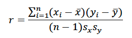
where n is the number of observations, i is an index, the overbar denotes average, and s is the sample standard deviation. sx is given by

and an equivalent formula exists for sy. The square of the Pearson correlation, r2 = the percent of variance in y explained by the linear relationship between x and y. If one then tries to use the independent variable to make a prediction of the behavior of y (yf is the forecast value vector for y), the resultant linear least squares regression line takes the form

where m is a function of the Pearson correlation and the quotient of the standard deviations

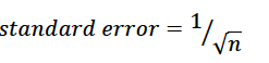
r values range from -1 to +1. r = -1 denotes a perfect inverse linear relationship between x and y (as x increases, y decreases in a predictable linear fashion); r = 0 denotes no linear relationship between x and y; r = 1 denotes a perfect direct linear relationship (as x increases, so does y in a predictable linear fashion). The statistical significance of the Pearson correlation depends on the number of observations and the correlation value. With relatively few observations strong correlations are easy to obtain but of limited value. The standard error statistic is given below
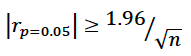
Generally a Pearson correlation value is considered “significant” at the 5% level for a two sided test if the absolute value of r is greater than 1.96 standard errors.
Note that correlation does not imply causation.
Mean bias: The mean bias is simply an indication of the difference between the average of the predicted value (yf) and the observed value (yo) of the variable in question. The simplest format for this is the difference format
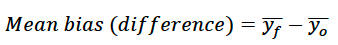
where, again, the overbar indicates average value. But mean bias can also be expressed in quotient format as the above difference divided by the average of the observed value, or

For climate related analyses, the quotient formulation is often used to express biases in rainfall and other “bounded” phenomena, whereas the difference formulation is often used to express biases in temperature and other “unbounded” phenomena. In other words, a climate model output might be said to have a 10% overestimate of rainfall, but a 2 deg C cool bias in temperature, relative to observations.
Mean Absolute Error (MAE): The mean absolute error or MAE is a metric of the absolute value of the average difference between the predicted and observed values.

Note that the mean absolute error will be greater than or equal to the mean bias. In general, the magnitude of the mean bias and mean absolute error are correlated to each other. But it is possible to have a large MAE with zero mean bias and it is possible to have the magnitude of the mean bias be equal to the MAE.
Root Mean Squared Error (RMSE): The root mean squared error or RMSE evaluates the square root of the square of the difference between predicted and observed values.
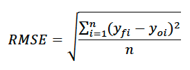
The RMSE is slightly more sensitive to large differences between observed and predicted values. Consider three pairs of observations and predictions where the absolute differences between them are 2, 6 and 10 units. The MAE is 6, whereas the RMSE = ((4+36+100)/3)1/2=6.8.
Linear Error in Probability Space (LEPS): One can also think of forecasts in probability space. For an individual prediction/observation pair, both the prediction and observation represent a value in the observed cumulative density function. If we consider both observed and predicted rainfall datasets with mean value 400 mm and standard deviation and a normal distribution, perhaps the observation of 350 mm is paired with a prediction of 360mm. The observation has a zscore value of (350-400)/50 = -1, and so the CDF value is about 0.16 or 16%. The prediction value has a z score of (360-400)/50 = -0.8 which corresponds to the CDF value of 21%. The LEPS value is the absolute difference between these CDF values or
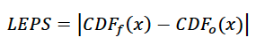
which, in this case is 0.05 or 5%. The LEPS statistic can be evaluated for each observation in the observational dataset and the average can be calculated. By virtue of the LEPS statistic being defined in absolute value terms, it is strictly non-negative and lower values of LEPS are preferable. Note that for given difference between observed and predicted values in the actual metric of measurement (rainfall, temperature, etc.), the LEPS score will be higher when the values in question are near the middle of the distribution than when the values are very large or very small. For example, with a similar example to the above, if the observation is 500mm and the forecast is 510mm, the absolute difference is the same as in the prior example (the forecast is 10mm too wet). However, in this case the 500mm observation represents a z score of +2 which takes a CDF value of 97.7%, while the forecast (510 mm) represents a zscore of +2.2 which takes a CDF value of 98.6%. So the LEPS value is 0.009 or 0.9%.
There is also a LEPS “skill score” which is 1-LEPS for which higher values, closer to 1 are optimal.
Discrete/Categorical skill metrics
2 Alternative Forced Choice (2AFC): The two alternative forced choice score or 2AFC for short determines how well a forecast characterizes values as being above or below the average. If both the forecast and the observations are above the average or both below the average for a given pair, this pair is said to be a “hit”. If the forecast is above the average and the observation is below the average, or vice versa (the forecast is below the average and the observation is above the average), that pair is considered a “miss”. The total number of pairs of observations in the dataset is n = hits+misses. The 2AFC score is given by
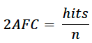
For normally or near-normally distributed data, the 2AFC score from random guessing would be about 50% or around 0.5. For strongly skewed data, the 2AFC score may converge on a different number as a function of the skew (i.e. for data with a strong rightward skew – eg. wealth), the random guessing 2AFC score for the lower category would be above 50% and the random guessing 2AFC score for the higher category would be below 50%. The 2AFC score should only be considered “good” if it is substantially higher than the level obtained by random guessing.
Hit Score (HS): The hit score or HS is similar to the 2AFC score, but is a more general form of it. The user can define a threshold of interest for the hit score – it doesn’t have to be the mean value. Again, the value is the hits/n.

Heidke Skill Score or Hit Skill Score (HSS): The HSS is a quotient where the numerator is the hit rate of the forecast minus the hit rate one would expect by chance. The denominator is the hit rate of a perfect forecast (1) minus the hit rate one would expect by chance. In the simplest case, we can consider the 2×2 contingency table below:
| Event observed | Event not observed | |
| Event forecast | a (hits) | b (false alarms) |
| Event not forecast | c (misses) | d (correct negatives) |
Intuitively, the success rate by chance is the
[(event forecast frequency)*(event observed frequency)+(event not forecast frequency)*(event not observed frequency)]/n2 =
[(a+b)(a+c)+(b+d)(c+d)]/n2
Using this equation, the understanding that n = a+b+c+d and some algebra, it can be shown that the Heidke or Hit Skill Score is
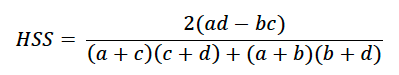
for such a 2×2 contingency table. Consider the probability of not exceeding the 20th percentile. If the forecast had no skill, but also no systematic bias, the four values in the contingency table were as follows: hits (a) = 0.04 or 4%, false alarms (b) = 0.16 or 16%, misses (c) = 0.16 or 16% and correct negatives (d) = 0.64 or 64%. So ad = 0.04*0.64 = 0.0256 = bc = 0.16*0.16 and the HSS = 0. If the forecast had positive skill (i.e. ad>bc), the HSS would be positive.
Relative Operating Characteristics (ROC): The relative operating characteristic and curve measures the hit rate to the false alarm rate of a classifier using different threshold settings in the predictive variable. In the ROC framework, the hit rate (hits/(hits+misses)) or (a/(a+c)) is plotted on the y axis, whereas the false alarm rate (false alarms/(false alarms+correct negatives)) or (b/(b+d)) is plotted on the x axis. It can be shown that if a forecast has no skill (is based on pure chance), the x,y coordinates will fall on the line y=x. For example, consider an event that has a 30% chance of occurrence and is forecast 30% of the time. If the forecast has no skill, the percentage of hits will be the product of these two: 30% of 30% = 9%. The percentage of misses will be the forecast percentage minus the hit percentage (30-9 = 21%). The percentage of false alarms will also be 21% and the percentage of correct negatives will be the remainder (100-21-21-9 = 49%). The hit rate is 9/21 and the false alarm rate = 21/49. Both are equal to 0.429.
If the forecast has negative skill (is worse than random guessing), the y coordinate (hit rate) will be worse than (lower than) the x value (false alarm rate) or “below” the y=x line. Forecasts with positive skill have hit rates greater than the false alarm rate (above the y=x line). A perfect forecast has no false alarms and only hits (0,1).
For each combination of predicted and observed data and threshold criteria, there is a specific coordinate in the ROC space. The “ROC curve” is calculated by choosing a specified threshold in the observations, but allowing the predicted threshold to vary from most restrictive to most permissive.
For example, if we have a predicted rainfall dataset pf and an observed rainfall data po, both with average rainfall 400mm and standard deviation 50 mm, some of the observations will fall below 320mm, which constitutes a fairly significant drought. If we were to set the drought “threshold” in the predicted dataset to 200mm, it’s highly unlikely that any prediction would be that low, so there would effectively be no “hits” and only “misses”. But there would also be no false alarms, where the predicted rainfall was below 200 mm, but the observed rainfall was above 320 mm. So this would map to the point (0,0) in ROC space. If we increase the threshold value in the predictor steadily, we start to assess how well the predictions match the observations and how many misses and false alarms there are. If we set the predictive threshold to a very high value (say 600 mm), every event will be predicted to be below that threshold, so there will be many false alarms (prediction below 600, but observations above 300), some hits (prediction below 600, but observations below 300), but zero misses (prediction above 600, but observations below 300) and zero true negatives (prediction above 600, but observations above 300). This scenario will map to the point (1,1) in ROC space. For thresholds of non-exceedance like drought, the “most restrictive” values are the lowest, whereas the “most permissive” are the highest. For thresholds of exceedance (like heavy rainfall or high temperature), the “most restrictive” values are the highest, whereas the “most permissive” are the lowest.
The example below shows an ROC curve for the above normal and below normal terciles of a forecast (i.e. the 67th%ile and the 33rd %ile). You can see that the overall performance for this forecast is better for the above average category.

Gerrity Skill Score (GSS): The Gerrity Skill Score is also used in a contingency matrix framework, where positive “weights” are applied to boxes where the predicted and observed categories match and negative weights are ascribed to the boxes where the predicted and observed categories disagree. The balance of the positive and negative weights are such that a forecast based on random guessing will have a GSS of 0. Fundamentally, the Gerrity Skill score is given by
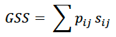
where the pij are the proportion of observations in each box and the sij are the weights. Let q be the number of categories in either direction of the contingency table. Let kappa = q-1. Let pr be the proportion of observations in category r. Indices i and j both have length r. The weights are calculated as follows. First another parameter “a” is calculated as follows.
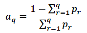
So for example, if we consider a two category framework and the probability of not exceeding the 20th percentile, a1 = (1-0.2)/0.2 = 4 and a2 = (1-1)/1 = 0.
Then for observations where the predicted and observed categories match, the weights are given by
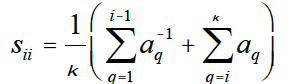
In the example above, kappa =1, so s11 = 4 and s22 = 1/4.
For j>i, observations where the j =/= i, the weights are given by

for i<j, sij = sji. So in the example above, s12=s21=-1. If the forecast had no skill, but also no systematic bias, the four values in the contingency table were as follows: hits (a) = 0.04 or 4%, false alarms (b) = 0.16 or 16%, misses (c) = 0.16 or 16% and correct negatives (d) = 0.64 or 64%. The GSS would then be 0.04*4+0.64/4-2*0.16 = 0. If the forecast had some positive skill (i.e. a>0.04 and d>0.64 and b and c were less than 0.16), the GSS would take a positive value.
Rank Skill Metrics
Spearman correlation: While often similar in value (and to some degree in meaning) to the Pearson correlation, the Spearman correlation value is based only n the ranks between the observed and predicted datasets. The data in the two datasets are ranked and the ranks are compared. The differences in rank are the di. So for example, if the predicted driest year is the observed driest year, the d for that individual year is 0, whereas if the predicted driest year is the third driest year, the di value is 2. The Spearman correlation is then given by the equation
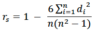
where n are the total number of data. As with the Pearson correlation, positive values denote positive linear correlation, while negative values denote negative linear correlation and values around 0 denote no significant correlation. If we consider x = [1 2 3 4 5] and y = [2 3 7 8 6], the ranks (considering larger values to be higher ranks) are x = [5 4 3 2 1] and y = [5 4 2 1 3]. So the di are 0, 0, 1, 1, -2 respectively. So the Spearman correlation is 1-36/(5*24) = 1-0.3 = 0.7.
Kendall Tau: The Kendall tau correlation is a sign-based correlation metric that seeks to understand the sign of the difference between different pairs of data within the dataset. The sign function (abbreviated below as sgn) takes the value of +1 for positive differences and -1 for negative differences. The Kendall tau statistic is given by

So when the differences between the ith and jth entry have the same sign (either both positive or both negative) for both the x and y datasets, the product of the sign functions will be +1, whereas when they have opposite signs, the product of the sign functions will be -1.
If we consider x = [1 2 3 4 5] and y = [2 3 7 8 6], we have, for ij = 1,2; 1,3; 1,4; 1,5; 2,3; 2,4; 2,5; and 3,4, sgn(xi-xj)sgn(yi-yj)=1. But for ij = 3,5; 4,5, sgn(xi-xj)sgn(yi-yj)=-1. So the sum = 8-2 = 6 and the Kendall tau value is 12/20=0.6.
Hybrid Skill metrics:
Brier Score (BS)/Brier Skill Score (BSS): The Brier score (BS) deals with binary events that either did happen (1) or didn’t (0). The Brier score is given by
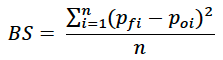
where the pfi is the forecast probability of the event and the poi is the outcome for that index value (either 0 or 1) and n is the total number of observations. So if we consider a dataset of five observations in which there was one “event” in the fourth position (i.e. po = [0 0 0 1 0]) and a relatively skillful forecast, where the forecast probabilities (in proportion terms) are pf = [0.2 0.2 0.1 0.7 0.4], the BS would be (0.04+0.04+0.01+0.09+0.16)/5 = 0.068. Because of the square in the numerator, the BS value is non-negative, but lower BS values are preferable.
The Brier skill score (or BSS) is simply

where BSf is the forecast Brier score and BSc is the Brier score for climatology. Higher BSS scores (closer to 1) are preferable. A BSS of 0 indicates the forecast is no better than random guessing. In our example from above, because the event occurs 20% of the time, the pc = [0.2 0.2 0.2 0.2 0.2] and BSc = (4*0.04+0.64)/5 = 0.16. Consequently, the BSS = 1-0.068/0.16 = 0.575 – which constitutes a significant improvement over random guessing. The Brier score and BSS can be considered “hybrid” because the forecast probabilities may be continuous, or may take discrete values.
Ranked Probability Score (RPS)/Ranked Probability Skill Score (RPSS): The ranked probability score (RPS) in a categorical sense is a somewhat more general version of the Brier score and calculates the difference between the cumulative probability density function of the forecasts and the cumulative probability density function of the observations. The equation is

where ncat is the number of categories and pcumcat is the probability that the forecast or observation is below the upper bound of that category and the subscript f stands for forecast and the subscript o stands for observations. Again the values for observations are either 0 or 1 – the event either did or did not happen. But the pcumcatf values can be continuous. Consider a forecast for an individual year’s rainfall based on terciles (the probability that the rainfall is below the 33rd %ile, between the 33rd and 67th %ile or above the 67th%ile). Let’s assume the forecast probabilities are (0.4, 0.3, 0.3) respectively (or 40% chance of below normal, 30% chance of near normal and 30% chance of above normal). The RPS for this individual forecast would then be ((0.4-0)2+(0.7-1)2+(1-1)2)/2 = 0.125. There is a continuous version of the RPS statistic (sometimes abbreviated CRPS) which considers an infinite number of categories, but essentially plots the same function and would be framed as an integral formula. As with the Brier Score, lower values of RPS are preferable, but the RPS statistic is strictly non-negative. As with the Brier score, the Ranked Probability Skill score is

where RPSf is the forecast RPS and RPSc is the climatological RPS. In our example above, the climatological RPSc = ((0.33-0)2+(0.67-1)2+(1-1)2)/2 = 0.109, so the RPSS is 1-0.125/0.109 = -0.147, so this forecast is slightly worse than random guessing. If the forecast had stayed the same, but the observation had been in the below normal category, the RPSf =((0.4-1)2+(0.7-1)2+(1-1)2)/2 = 0.225 and the RPSc = ((0.33-1)2+(0.67-1)2+(1-1)2)/2 = 0.279 and the RPSS would be 1-0.225/0.279 = 0.194.
R script
# This script yields a wide range of skill metrics for chosen x, yobs and ypred data. Ypred here is derived from x plus an error term. The user only needs to modify n, x, yo, ypred, the threshold percentages (lines 55 and 56), and maybe the forecast probabilities for Brier and Ranked Probability Scores near the end.
library('plyr')
n = 30
x <- c(25.5,	23.1,	24.6,	25.3,	22.3,	23.8,	26.3,	24.7,	26.4,	23.3,	21.5,	23.4,	25.7,	26.9,	24.9,	25.9,	27.4,	23,	25.2,	24.3,	27.7,	23.2,	23.3,	24.7,	29.5,	22.3,	26.2,	24.8,	25.8,	24.9)
yo <- c(1056,	1202,	1252,	1019,	946,	1190,	1107,	1168,	1075,	1103,	1032,	964,	1072,	1159,	1165,	1224,	1383,	911,	1040,	1000,	1174,	1199,	1053,	1209,	1428,	949,	1318,	1052,	1271,	1252)
xmean = sum(x)/n
yomean = sum(yo)/n
xsd = sd(x)
yosd = sd(yo)
#calculate Pearson r
r = (sum((x-xmean)*(yo-yomean)))/((n-1)*xsd*yosd)
print(paste('r',r))
#calculate OLS regression line and predicted y values
m = r*yosd/xsd
b = yomean-m*xmean
print(paste('m',m))
print(paste('b',b))
ypred = m*x+b
print(ypred)
ypredmean = sum(ypred)/n
#calculate threshold for 2 sided 5% significance/95% confidence
rthresh = 1.96/(n^0.5)
print(paste('rthresh',rthresh))
#calculate mean bias
meanbiasdiff = ypredmean-yomean
meanbiasprop = ypredmean/yomean-1
print(paste('meanbiasdiff',meanbiasdiff))
print(paste('meanbiasprop',meanbiasprop))
#calculate mean absolute error and root mean squared error
MAE = sum(abs(ypred-yo))/n
RMSE = sqrt((sum((ypred-yo)^2)/n))
print(paste('MAE',MAE))
print(paste('RMSE',RMSE))
#calculate LEPS from data and observed normal distribution
zscorepred = (ypred-yomean)/yosd
zscoreobs = (yo-yomean)/yosd
CDFf = pnorm(zscorepred)
CDFo = pnorm(zscoreobs)
LEPS = abs(CDFf-CDFo)
LEPSave = sum(LEPS)/n
LEPSSS = 1-LEPS
LEPSSSave = 1-LEPSave
print(LEPS)
print(paste('LEPSave',LEPSave))
print(LEPSSS)
print(paste('LEPSSSave',LEPSSSave))
#calculate 2AFC, Hit Score and Hit Skill Score/Heidke Skill Score
hithigh = sum(ifelse(ypred>ypredmean & yo>yomean, 1, 0))
print(paste('hithigh',hithigh))
hitlow = sum(ifelse(ypred<ypredmean & yo<yomean, 1, 0))
print(paste('hitlow',hitlow))
twoAFC <- (hithigh+hitlow)/n
print(paste('twoAFC',twoAFC))
#specify thresholds
highthreshperc = 80
lowthreshperc = 20
highthresh = quantile(yo,highthreshperc/100)
lowthresh = quantile(yo,lowthreshperc/100)
print(highthresh)
print(lowthresh)
#a = hits, b = false alarms, c = misses, d = true negatives
ahigh = sum(ifelse(ypred>=highthresh & yo>=highthresh, 1, 0))
print(paste('ahigh',ahigh))
bhigh = sum(ifelse(ypred>=highthresh & yo<highthresh, 1, 0))
print(paste('bhigh',bhigh))
chigh = sum(ifelse(ypred<=highthresh & yo>highthresh, 1, 0))
print(paste('chigh',chigh))
dhigh = sum(ifelse(ypred<highthresh & yo<highthresh, 1, 0))
print(paste('dhigh',dhigh))
alow = sum(ifelse(ypred<=lowthresh & yo<=lowthresh, 1, 0))
print(paste('alow',alow))
blow = sum(ifelse(ypred<=lowthresh & yo>lowthresh, 1, 0))
print(paste('blow',blow))
clow = sum(ifelse(ypred>=lowthresh & yo<=lowthresh, 1, 0))
print(paste('clow',clow))
dlow = sum(ifelse(ypred>lowthresh & yo>lowthresh, 1, 0))
print(paste('dlow',dlow))
HShigh = (ahigh+dhigh)/n
HSlow = (alow+dlow)/n
print(paste('HShigh',HShigh))
print(paste('HSlow',HSlow))
HSShigh = 2*(ahigh*dhigh-bhigh*chigh)/((ahigh+chigh)*(chigh+dhigh)+(ahigh+bhigh)*(bhigh+dhigh))
HSSlow = 2*(alow*dlow-blow*clow)/((alow+clow)*(clow+dlow)+(alow+blow)*(blow+dlow))
print(paste('HSShigh',HSShigh))
print(paste('HSSlow',HSSlow))
#calculate Gerrity skill score with same threshold and two by two contingency
p11high = ahigh/n
p12high = bhigh/n
p21high = chigh/n
p22high = dhigh/n
p11low = alow/n
p12low = blow/n
p21low = clow/n
p22low = dlow/n
s11high = highthreshperc/(100-highthreshperc)
s22high = (100-highthreshperc)/highthreshperc
s21high = s12high = -1
s11low = (100-lowthreshperc)/lowthreshperc
s22low = lowthreshperc/(100-lowthreshperc)
s21low = s12low = -1
GSShigh=p11high*s11high+p12high*s12high+p21high*s21high+p22high*s22high
GSSlow=p11low*s11low+p12low*s12low+p21low*s21low+p22low*s22low
print(paste('GSShigh',GSShigh))
print(paste('GSSlow',GSSlow))
#calculate ROC curve and area across thresholds by deciles
highthreshpercROC = c(100,90,80,70,60,50,40,30,20,10,0)
lowthreshpercROC = c(0,10,20,30,40,50,60,70,80,90,100)
highthreshROC = quantile(ypred,highthreshpercROC/100)
lowthreshROC = quantile(ypred,lowthreshpercROC/100)
print(highthreshROC)
print(lowthreshROC)
#a = hits, b = false alarms, c = misses, d = true negatives
ahighROC <- matrix(NA,1,11)
for (i in 1:11) {ahighROC[i] = sum(ifelse(ypred>=highthreshROC[i] & yo>=highthresh, 1, 0))}
print(ahighROC)
bhighROC <- matrix(NA,1,11)
for (i in 1:11) {bhighROC[i] = sum(ifelse(ypred>=highthreshROC[i] & yo<highthresh, 1, 0))}
print(bhighROC)
chighROC <- matrix(NA,1,11)
for (i in 1:11) {chighROC[i] = sum(ifelse(ypred<highthreshROC[i] & yo>=highthresh, 1, 0))}
print(chighROC)
dhighROC <- matrix(NA,1,11)
for (i in 1:11) {dhighROC[i] = sum(ifelse(ypred<highthreshROC[i] & yo<highthresh, 1, 0))}
print(dhighROC)
alowROC <- matrix(NA,1,11)
for (i in 1:11) {alowROC[i] = sum(ifelse(ypred<=lowthreshROC[i] & yo<=lowthresh, 1, 0))}
print(alowROC)
blowROC <- matrix(NA,1,11)
for (i in 1:11) {blowROC[i] = sum(ifelse(ypred<=lowthreshROC[i] & yo>lowthresh, 1, 0))}
print(blowROC)
clowROC <- matrix(NA,1,11)
for (i in 1:11) {clowROC[i] = sum(ifelse(ypred>lowthreshROC[i] & yo<=lowthresh, 1, 0))}
print(clowROC)
dlowROC <- matrix(NA,1,11)
for (i in 1:11) {dlowROC[i] = sum(ifelse(ypred>lowthreshROC[i] & yo>lowthresh, 1, 0))}
print(dlowROC)
ROCyhigh = ahighROC/(ahighROC+chighROC)
ROCxhigh = bhighROC/(bhighROC+dhighROC)
ROCylow = alowROC/(alowROC+clowROC)
ROCxlow = blowROC/(blowROC+dlowROC)
print(ROCyhigh)
print(ROCxhigh)
print(ROCylow)
print(ROCxlow)
plot(ROCxhigh, ROCyhigh, type="l", col="blue", pch="o", lty=1, ylim=c(0,1), main = "ROC", xlab = "proportion of false alarms", ylab = "proportion of hits")
lines(ROCxlow, ROCylow, col="green")
lines(ROCxhigh, ROCxhigh, col="black")
legend(0.45, 0.3, legend=c("high threshold", "low threshold","no skill"), fill = c("blue","green","black"))
ROCyhighave = c((ROCyhigh[2]+ROCyhigh[1])/2,(ROCyhigh[3]+ROCyhigh[2])/2,(ROCyhigh[4]+ROCyhigh[3])/2,(ROCyhigh[5]+ROCyhigh[4])/2,(ROCyhigh[6]+ROCyhigh[5])/2,(ROCyhigh[7]+ROCyhigh[6])/2,(ROCyhigh[8]+ROCyhigh[7])/2,(ROCyhigh[9]+ROCyhigh[8])/2,(ROCyhigh[10]+ROCyhigh[9])/2,(ROCyhigh[11]+ROCyhigh[10])/2)
ROCxhighdiff = c(ROCxhigh[2]-ROCxhigh[1],ROCxhigh[3]-ROCxhigh[2],ROCxhigh[4]-ROCxhigh[3],ROCxhigh[5]-ROCxhigh[4],ROCxhigh[6]-ROCxhigh[5],ROCxhigh[7]-ROCxhigh[6],ROCxhigh[8]-ROCxhigh[7],ROCxhigh[9]-ROCxhigh[8],ROCxhigh[10]-ROCxhigh[9],ROCxhigh[11]-ROCxhigh[10])
ROCylowave = c((ROCylow[2]+ROCylow[1])/2,(ROCylow[3]+ROCylow[2])/2,(ROCylow[4]+ROCylow[3])/2,(ROCylow[5]+ROCylow[4])/2,(ROCylow[6]+ROCylow[5])/2,(ROCylow[7]+ROCylow[6])/2,(ROCylow[8]+ROCylow[7])/2,(ROCylow[9]+ROCylow[8])/2,(ROCylow[10]+ROCylow[9])/2,(ROCylow[11]+ROCylow[10])/2)
ROCxlowdiff = c(ROCxlow[2]-ROCxlow[1],ROCxlow[3]-ROCxlow[2],ROCxlow[4]-ROCxlow[3],ROCxlow[5]-ROCxlow[4],ROCxlow[6]-ROCxlow[5],ROCxlow[7]-ROCxlow[6],ROCxlow[8]-ROCxlow[7],ROCxlow[9]-ROCxlow[8],ROCxlow[10]-ROCxlow[9],ROCxlow[11]-ROCxlow[10])
ROChigh = sum(ROCyhighave*ROCxhighdiff)
ROClow = sum(ROCylowave*ROCxlowdiff)
print(paste('ROChigh',ROChigh))
print(paste('ROClow',ROClow))
#calculate Spearman rank correlation
yorank = rank(yo)
ypredrank = rank(ypred)
d = ypredrank-yorank
rs = 1-6*sum(d^2)/(n*(n^2-1))
print(paste('rspearman',rs))
#calculate Kendall tau
tausign2 = matrix(NA,1,1)
for (i in 1:1) {tausign2[i] = (x[i]-x[2])*(yo[i]-yo[2])}
tau2 = sum(ifelse(tausign2>0,1,-1))
tausign3 = matrix(NA,1,2)
for (i in 1:2) {tausign3[i] = (x[i]-x[3])*(yo[i]-yo[3])}
tau3 = sum(ifelse(tausign3>0,1,-1))
tausign4 = matrix(NA,1,3)
for (i in 1:3) {tausign4[i] = (x[i]-x[4])*(yo[i]-yo[4])}
tau4 = sum(ifelse(tausign4>0,1,-1))
tausign5 = matrix(NA,1,4)
for (i in 1:4) {tausign5[i] = (x[i]-x[5])*(yo[i]-yo[5])}
tau5 = sum(ifelse(tausign5>0,1,-1))
tausign6 = matrix(NA,1,5)
for (i in 1:5) {tausign6[i] = (x[i]-x[6])*(yo[i]-yo[6])}
tau6 = sum(ifelse(tausign6>0,1,-1))
tausign7 = matrix(NA,1,6)
for (i in 1:6) {tausign7[i] = (x[i]-x[7])*(yo[i]-yo[7])}
tau7 = sum(ifelse(tausign7>0,1,-1))
tausign8 = matrix(NA,1,7)
for (i in 1:7) {tausign8[i] = (x[i]-x[8])*(yo[i]-yo[8])}
tau8 = sum(ifelse(tausign8>0,1,-1))
tausign9 = matrix(NA,1,8)
for (i in 1:8) {tausign9[i] = (x[i]-x[9])*(yo[i]-yo[9])}
tau9 = sum(ifelse(tausign9>0,1,-1))
tausign10 = matrix(NA,1,9)
for (i in 1:9) {tausign10[i] = (x[i]-x[10])*(yo[i]-yo[10])}
tau10 = sum(ifelse(tausign10>0,1,-1))
tausign11 = matrix(NA,1,10)
for (i in 1:10) {tausign11[i] = (x[i]-x[11])*(yo[i]-yo[11])}
tau11 = sum(ifelse(tausign11>0,1,-1))
tausign12 = matrix(NA,1,11)
for (i in 1:11) {tausign12[i] = (x[i]-x[12])*(yo[i]-yo[12])}
tau12 = sum(ifelse(tausign12>0,1,-1))
tausign13 = matrix(NA,1,12)
for (i in 1:12) {tausign13[i] = (x[i]-x[13])*(yo[i]-yo[13])}
tau13 = sum(ifelse(tausign13>0,1,-1))
tausign14 = matrix(NA,1,13)
for (i in 1:13) {tausign14[i] = (x[i]-x[14])*(yo[i]-yo[14])}
tau14 = sum(ifelse(tausign14>0,1,-1))
tausign15 = matrix(NA,1,14)
for (i in 1:14) {tausign15[i] = (x[i]-x[15])*(yo[i]-yo[15])}
tau15 = sum(ifelse(tausign15>0,1,-1))
tausign16 = matrix(NA,1,15)
for (i in 1:15) {tausign16[i] = (x[i]-x[16])*(yo[i]-yo[16])}
tau16 = sum(ifelse(tausign16>0,1,-1))
tausign17 = matrix(NA,1,16)
for (i in 1:16) {tausign17[i] = (x[i]-x[17])*(yo[i]-yo[17])}
tau17 = sum(ifelse(tausign17>0,1,-1))
tausign18 = matrix(NA,1,17)
for (i in 1:17) {tausign18[i] = (x[i]-x[18])*(yo[i]-yo[18])}
tau18 = sum(ifelse(tausign18>0,1,-1))
tausign19 = matrix(NA,1,18)
for (i in 1:18) {tausign19[i] = (x[i]-x[19])*(yo[i]-yo[19])}
tau19 = sum(ifelse(tausign19>0,1,-1))
tausign20 = matrix(NA,1,19)
for (i in 1:19) {tausign20[i] = (x[i]-x[20])*(yo[i]-yo[20])}
tau20 = sum(ifelse(tausign20>0,1,-1))
tausign21 = matrix(NA,1,20)
for (i in 1:20) {tausign21[i] = (x[i]-x[21])*(yo[i]-yo[21])}
tau21 = sum(ifelse(tausign21>0,1,-1))
tausign22 = matrix(NA,1,21)
for (i in 1:21) {tausign22[i] = (x[i]-x[22])*(yo[i]-yo[22])}
tau22 = sum(ifelse(tausign22>0,1,-1))
tausign23 = matrix(NA,1,22)
for (i in 1:22) {tausign23[i] = (x[i]-x[23])*(yo[i]-yo[23])}
tau23 = sum(ifelse(tausign23>0,1,-1))
tausign24 = matrix(NA,1,23)
for (i in 1:23) {tausign24[i] = (x[i]-x[24])*(yo[i]-yo[24])}
tau24 = sum(ifelse(tausign24>0,1,-1))
tausign25 = matrix(NA,1,24)
for (i in 1:24) {tausign25[i] = (x[i]-x[25])*(yo[i]-yo[25])}
tau25 = sum(ifelse(tausign25>0,1,-1))
tausign26 = matrix(NA,1,25)
for (i in 1:25) {tausign26[i] = (x[i]-x[26])*(yo[i]-yo[26])}
tau26 = sum(ifelse(tausign26>0,1,-1))
tausign27 = matrix(NA,1,26)
for (i in 1:26) {tausign27[i] = (x[i]-x[27])*(yo[i]-yo[27])}
tau27 = sum(ifelse(tausign27>0,1,-1))
tausign28 = matrix(NA,1,27)
for (i in 1:27) {tausign28[i] = (x[i]-x[28])*(yo[i]-yo[28])}
tau28 = sum(ifelse(tausign28>0,1,-1))
tausign29 = matrix(NA,1,28)
for (i in 1:28) {tausign29[i] = (x[i]-x[29])*(yo[i]-yo[29])}
tau29 = sum(ifelse(tausign29>0,1,-1))
tausign30 = matrix(NA,1,29)
for (i in 1:29) {tausign30[i] = (x[i]-x[30])*(yo[i]-yo[30])}
tau30 = sum(ifelse(tausign30>0,1,-1))
tau = tau2+tau3+tau4+tau5+tau6+tau7+tau8+tau9+tau10+tau11+tau12+tau13+tau14+tau15+tau16+tau17+tau18+tau19+tau20+tau21+tau22+tau23+tau24+tau25+tau26+tau27+tau28+tau29+tau30
ktau = (2/(n*(n-1)))*tau
print(paste('tau',tau))
print(paste('ktau',ktau))
#calculate Brier scores and Brier Skill Scores with chosen thresholds, forecast probability based on normal distribution assumption and ypred being the mean of the forecast distribution
POhigh = ifelse(yo>=highthresh,1,0)
PChigh = c(rep(1-highthreshperc/100,n))
POlow = ifelse(yo<=lowthresh,1,0)
PClow = c(rep(lowthreshperc/100,n))
zscorehighthresh = (highthresh-yomean)/yosd
zscorelowthresh = (lowthresh-yomean)/yosd
zscorediffhigh = zscorehighthresh-zscorepred
zscoredifflow = zscorelowthresh-zscorepred
PFhigh = 1-pnorm(zscorediffhigh)
PFlow = pnorm(zscoredifflow)
BShigh = (sum((PFhigh-POhigh)^2))/n
BShighc = (sum((PChigh-POhigh)^2))/n
BSlow = (sum((PFlow-POlow)^2))/n
BSlowc = (sum((PClow-POlow)^2))/n
print(paste('BShigh',BShigh))
print(paste('BSlow',BSlow))
BSShigh = 1-BShigh/BShighc
BSSlow = 1-BSlow/BSlowc
print(paste('BSShigh',BSShigh))
print(paste('BSSlow',BSSlow))
#calculate the rank probability score and the rank probability skill score with terciles - again with forecast probability based on normal distribution assumption and ypred being mean of forecast distribution
lowterc = quantile(yo,0.33)
highterc = quantile(yo,0.67)
zscorelowterc = (lowterc-yomean)/yosd
zscorehighterc = (highterc-yomean)/yosd
polow = ifelse(yo<=lowterc,1,0)
pomid = ifelse(yo<=highterc,1,0)
pohigh = c(rep(1,n))
po = matrix(NA,3,n)
po[1,] = polow
po[2,] = pomid
po[3,] = pohigh
#print(po)
pflow = pnorm(zscorelowterc-zscorepred)
pfmid = pnorm(zscorehighterc-zscorepred)
pfhigh = c(rep(1,n))
pf = matrix(NA,3,n)
pf[1,] = pflow
pf[2,] = pfmid
pf[3,] = pfhigh
#print(pf)
pc = matrix(NA,3,n)
pc[1,] = c(rep(0.33,n))
pc[2,] = c(rep(0.67,n))
pc[3,] = c(rep(1,n))
#print(pc)
RPSf = (1/(2*n))*sum((pf-po)^2)
print(paste('RPSf',RPSf))
RPSc = (1/(2*n))*sum((pc-po)^2)
print(paste('RPSc',RPSc))
RPSS = 1-RPSf/RPSc
print(paste('RPSS',RPSS))</code>
Python script
#Continuous skill metrics
# This script yields a wide range of skill metrics for chosen x, yobs and ypred data.Ypred here is derived from x plus an error term.
import pandas as pd
import numpy as np
import scipy.stats as stats
import matplotlib.pyplot as plt

n = 30
x = [25.5,23.1,24.6,25.3,22.3,23.8,26.3,24.7,26.4,23.3,21.5,23.4,25.7,26.9,24.9,25.9,27.4,23,25.2,24.3,27.7,23.2,23.3,24.7,29.5,22.3,26.2,24.8,25.8,24.9]
yo = [1056,1202,1252,1019,946,1190,1107,1168,1075,1103,1032,964,1072,1159,1165,1224,1383,911,1040,1000,1174,1199,1053,1209,1428,949,1318,1052,1271,1252]
xmean = sum(x)/n
yomean = sum(yo)/n
xsd = np.std(x)
yosd = np.std(yo)
#calculate Pearson r
r = sum((np.multiply((np.subtract(x,xmean)),(np.subtract(yo,yomean))))/((n-1)*xsd*yosd))
print('r',r)
#calculate OLS regression line and predicted y values
m = r*yosd/xsd
b = yomean-m*xmean
print('m',m)
print('b',b)
ypred = np.multiply(m,x)+b
print(ypred)
ypredmean = sum(ypred)/n
#calculate threshold for 2 sided 5% significance/95% confidence
rthresh = 1.96/(n**0.5)
print('rthresh',rthresh)
#calculate mean bias
meanbiasdiff = ypredmean-yomean
meanbiasprop = ypredmean/yomean-1
print('meanbiasdiff',meanbiasdiff)
print('meanbiasprop',meanbiasprop)
#calculate mean absolute error and root mean squared error
MAE = sum(abs(ypred-yo))/n
RMSE = (sum((ypred-yo)**2)/n)**0.5
print('MAE',MAE)
print('RMSE',RMSE)
#calculate LEPS from data and observed normal distribution
zscorepred = (np.subtract(ypred,yomean))/yosd
zscoreobs = (np.subtract(yo,yomean))/yosd
CDFf = stats.norm.cdf(zscorepred)
CDFo = stats.norm.cdf(zscoreobs)
LEPS = abs(CDFf-CDFo)
LEPSave = sum(LEPS)/n
LEPSSS = 1-LEPS
LEPSSSave = 1-LEPSave
print(LEPS)
print('LEPSave',LEPSave)
print(LEPSSS)
print('LEPSSSave',LEPSSSave)
#Discrete scores
#calculate 2AFC, Hit Score and Hit Skill Score/Heidke Skill Score
hithigh = sum(np.greater_equal(ypred,ypredmean) & np.greater_equal(yo,yomean))
print('hithigh',hithigh)
hitlow = sum(np.less(ypred,ypredmean) & np.less(yo,yomean))
print('hitlow',hitlow)
twoAFC = (hithigh+hitlow)/n
print('twoAFC',twoAFC)
#specify thresholds
highthreshperc = 80
lowthreshperc = 20
highthresh = np.quantile(yo,highthreshperc/100)
lowthresh = np.quantile(yo,lowthreshperc/100)
print(highthresh)
print(lowthresh)
#a = hits, b = false alarms, c = misses, d = true negatives
ahigh = sum(np.greater_equal(ypred,highthresh) & np.greater_equal(yo,highthresh))
print('ahigh',ahigh)
bhigh = sum(np.greater_equal(ypred,highthresh) & np.less(yo,highthresh))
print('bhigh',bhigh)
chigh = sum(np.less(ypred,highthresh) & np.greater_equal(yo,highthresh))
print('chigh',chigh)
dhigh = sum(np.less(ypred,highthresh) & np.less(yo,highthresh))
print('dhigh',dhigh)
alow = sum(np.less_equal(ypred,lowthresh) & np.less_equal(yo,lowthresh))
print('alow',alow)
blow = sum(np.less_equal(ypred,lowthresh) & np.greater(yo,lowthresh))
print('blow',blow)
clow = sum(np.greater(ypred,lowthresh) & np.less_equal(yo,lowthresh))
print('clow',clow)
dlow = sum(np.greater(ypred,lowthresh) & np.greater(yo,lowthresh))
print('dlow',dlow)
HShigh = (ahigh+dhigh)/n
HSlow = (alow+dlow)/n
print('HShigh',HShigh)
print('HSlow',HSlow)
HSShigh = 2*(ahigh*dhigh-bhigh*chigh)/((ahigh+chigh)*(chigh+dhigh)+(ahigh+bhigh)*(bhigh+dhigh))
HSSlow = 2*(alow*dlow-blow*clow)/((alow+clow)*(clow+dlow)+(alow+blow)*(blow+dlow))
print('HSShigh',HSShigh)
print('HSSlow',HSSlow)
#calculate Gerrity skill score with same threshold and two by two contingency
p11high = ahigh/n
p12high = bhigh/n
p21high = chigh/n
p22high = dhigh/n
p11low = alow/n
p12low = blow/n
p21low = clow/n
p22low = dlow/n
s11high = highthreshperc/(100-highthreshperc)
s22high = (100-highthreshperc)/highthreshperc
s21high = s12high = -1
s11low = (100-lowthreshperc)/lowthreshperc
s22low = lowthreshperc/(100-lowthreshperc)
s21low = s12low = -1
GSShigh=p11high*s11high+p12high*s12high+p21high*s21high+p22high*s22high
GSSlow=p11low*s11low+p12low*s12low+p21low*s21low+p22low*s22low
print('GSShigh',GSShigh)
print('GSSlow',GSSlow)
#ROC
#calculate ROC curve and area across thresholds by deciles
highthreshpercROC = [100,90,80,70,60,50,40,30,20,10,0]
lowthreshpercROC = [0,10,20,30,40,50,60,70,80,90,100]
HIGHTHRESH = np.repeat(highthresh,11)
LOWTHRESH = np.repeat(lowthresh,11)
highthreshROC = np.quantile(ypred,np.divide(highthreshpercROC,100))
lowthreshROC = np.quantile(ypred,np.divide(lowthreshpercROC,100))
print(highthreshROC)
print(lowthreshROC)
#a = hits, b = false alarms, c = misses, d = true negatives
ahighROC = np.zeros((1,11))
for i in range(1,12):
    ahighROC[0,i-1] = sum(np.greater_equal(ypred,highthreshROC[i-1]) & np.greater_equal(yo,HIGHTHRESH[i-1]))
print('ahighROC',ahighROC)
bhighROC = np.zeros((1,11))
for i in range(1,12):
    bhighROC[0,i-1] = sum(np.greater_equal(ypred,highthreshROC[i-1]) & np.less(yo,HIGHTHRESH[i-1]))
print('bhighROC',bhighROC)
chighROC = np.zeros((1,11))
for i in range(1,12):
    chighROC[0,i-1] = sum(np.less(ypred,highthreshROC[i-1]) & np.greater_equal(yo,HIGHTHRESH[i-1]))
print('chighROC',chighROC)
dhighROC = np.zeros((1,11))
for i in range(1,12):
    dhighROC[0,i-1] = sum(np.less(ypred,highthreshROC[i-1]) & np.less(yo,HIGHTHRESH[i-1]))
print('dhighROC',dhighROC)
alowROC = np.zeros((1,11))
for i in range(1,12):
    alowROC[0,i-1] = sum(np.less_equal(ypred,lowthreshROC[i-1]) & np.less_equal(yo,LOWTHRESH[i-1]))
print('alowROC',alowROC)
blowROC = np.zeros((1,11))
for i in range(1,12):
    blowROC[0,i-1] = sum(np.less_equal(ypred,lowthreshROC[i-1]) & np.greater(yo,LOWTHRESH[i-1]))
print('blowROC',blowROC)
clowROC = np.zeros((1,11))
for i in range(1,12):
    clowROC[0,i-1] = sum(np.greater(ypred,lowthreshROC[i-1]) & np.less_equal(yo,LOWTHRESH[i-1]))
print('clowROC',clowROC)
dlowROC = np.zeros((1,11))
for i in range(1,12):
    dlowROC[0,i-1] = sum(np.greater(ypred,lowthreshROC[i-1]) & np.greater(yo,LOWTHRESH[i-1]))
print('dlowROC',dlowROC)
ROCyhigh = ahighROC/(ahighROC+chighROC)
ROCxhigh = bhighROC/(bhighROC+dhighROC)
ROCylow = alowROC/(alowROC+clowROC)
ROCxlow = blowROC/(blowROC+dlowROC)
print(ROCyhigh)
print(ROCxhigh)
print(ROCylow)
print(ROCxlow)
plt.title('ROC curve')
plt.xlabel('false alarm ratio')
plt.ylabel('hit ratio')
plt.plot(np.transpose(ROCxhigh), np.transpose(ROCyhigh), label = "high")
plt.plot(np.transpose(ROCxlow), np.transpose(ROCylow), label = "low")
plt.legend()
plt.show()
ROCyhighave = [(ROCyhigh[0,1]+ROCyhigh[0,0])/2,(ROCyhigh[0,2]+ROCyhigh[0,1])/2,(ROCyhigh[0,3]+ROCyhigh[0,2])/2,(ROCyhigh[0,4]+ROCyhigh[0,3])/2,(ROCyhigh[0,5]+ROCyhigh[0,4])/2,(ROCyhigh[0,6]+ROCyhigh[0,5])/2,(ROCyhigh[0,7]+ROCyhigh[0,6])/2,(ROCyhigh[0,8]+ROCyhigh[0,7])/2,(ROCyhigh[0,9]+ROCyhigh[0,8])/2,(ROCyhigh[0,10]+ROCyhigh[0,9])/2]
ROCxhighdiff = [ROCxhigh[0,1]-ROCxhigh[0,0],ROCxhigh[0,2]-ROCxhigh[0,1],ROCxhigh[0,3]-ROCxhigh[0,2],ROCxhigh[0,4]-ROCxhigh[0,3],ROCxhigh[0,5]-ROCxhigh[0,4],ROCxhigh[0,6]-ROCxhigh[0,5],ROCxhigh[0,7]-ROCxhigh[0,6],ROCxhigh[0,8]-ROCxhigh[0,7],ROCxhigh[0,9]-ROCxhigh[0,8],ROCxhigh[0,10]-ROCxhigh[0,9]]
ROCylowave = [(ROCylow[0,1]+ROCylow[0,0])/2,(ROCylow[0,2]+ROCylow[0,1])/2,(ROCylow[0,3]+ROCylow[0,2])/2,(ROCylow[0,4]+ROCylow[0,3])/2,(ROCylow[0,5]+ROCylow[0,4])/2,(ROCylow[0,6]+ROCylow[0,5])/2,(ROCylow[0,7]+ROCylow[0,6])/2,(ROCylow[0,8]+ROCylow[0,7])/2,(ROCylow[0,9]+ROCylow[0,8])/2,(ROCylow[0,10]+ROCylow[0,9])/2]
ROCxlowdiff = [ROCxlow[0,1]-ROCxlow[0,0],ROCxlow[0,2]-ROCxlow[0,1],ROCxlow[0,3]-ROCxlow[0,2],ROCxlow[0,4]-ROCxlow[0,3],ROCxlow[0,5]-ROCxlow[0,4],ROCxlow[0,6]-ROCxlow[0,5],ROCxlow[0,7]-ROCxlow[0,6],ROCxlow[0,8]-ROCxlow[0,7],ROCxlow[0,9]-ROCxlow[0,8],ROCxlow[0,10]-ROCxlow[0,9]]
print(ROCyhighave)
print(ROCxhighdiff)
print(ROCylowave)
print(ROCxlowdiff)
ROChigh = sum(np.multiply(ROCyhighave,ROCxhighdiff))
ROClow = sum(np.multiply(ROCylowave,ROCxlowdiff))
print('ROChigh',ROChigh)
print('ROClow',ROClow)
#calculate Spearman rank correlation
yorank = np.argsort(yo)
ypredrank = np.argsort(ypred)
d = ypredrank-yorank
rs = 1-6*sum(d**2)/(n*(n**2-1))
print('rspearman',rs)
#calculate Kendall tau
tausign2 = np.zeros((1,1))
for i in range(1,1):
    tausign2[i] = (x[i-1]-x[1])*(yo[i-1]-yo[1])
tausign3 = np.zeros((2,1))
for i in range(1,2):
    tausign3[i] = (x[i-1]-x[2])*(yo[i-1]-yo[2])
tausign4 = np.zeros((3,1))
for i in range(1,3):
    tausign4[i] = (x[i-1]-x[3])*(yo[i-1]-yo[3])
tausign5 = np.zeros((4,1))
for i in range(1,4):
    tausign5[i] = (x[i-1]-x[4])*(yo[i-1]-yo[4])
tausign6 = np.zeros((5,1))
for i in range(1,5):
    tausign6[i] = (x[i-1]-x[5])*(yo[i-1]-yo[5])
tausign7 = np.zeros((6,1))
for i in range(1,6):
    tausign7[i] = (x[i-1]-x[6])*(yo[i-1]-yo[6])
tausign8 = np.zeros((7,1))
for i in range(1,7):
    tausign8[i] = (x[i-1]-x[7])*(yo[i-1]-yo[7])
tausign9 = np.zeros((8,1))
for i in range(1,8):
    tausign9[i] = (x[i-1]-x[8])*(yo[i-1]-yo[8])
tausign10 = np.zeros((9,1))
for i in range(1,9):
    tausign10[i] = (x[i-1]-x[9])*(yo[i-1]-yo[9])
tausign11 = np.zeros((10,1))
for i in range(1,10):
    tausign11[i] = (x[i-1]-x[10])*(yo[i-1]-yo[10])
tausign12 = np.zeros((11,1))
for i in range(11,1):
    tausign12[i] = (x[i-1]-x[11])*(yo[i-1]-yo[11])
tausign13 = np.zeros((12,1))
for i in range(1,12):
    tausign13[i] = (x[i-1]-x[12])*(yo[i-1]-yo[12])
tausign14 = np.zeros((13,1))
for i in range(1,13):
    tausign14[i] = (x[i-1]-x[13])*(yo[i-1]-yo[13])
tausign15 = np.zeros((14,1))
for i in range(1,14):
    tausign15[i] = (x[i-1]-x[14])*(yo[i-1]-yo[14])
tausign16 = np.zeros((15,1))
for i in range(1,15):
    tausign16[i] = (x[i-1]-x[15])*(yo[i-1]-yo[15])
tausign17 = np.zeros((16,1))
for i in range(1,16):
    tausign17[i] = (x[i-1]-x[16])*(yo[i-1]-yo[16])
tausign18 = np.zeros((17,1))
for i in range(1,17):
    tausign18[i] = (x[i-1]-x[17])*(yo[i-1]-yo[17])
tausign19 = np.zeros((18,1))
for i in range(1,18):
    tausign19[i] = (x[i-1]-x[18])*(yo[i-1]-yo[18])
tausign20 = np.zeros((19,1))
for i in range(1,19):
    tausign20[i] = (x[i-1]-x[19])*(yo[i-1]-yo[19])
tausign21 = np.zeros((20,1))
for i in range(1,20):
    tausign21[i] = (x[i-1]-x[20])*(yo[i-1]-yo[20])
tausign22 = np.zeros((21,1))
for i in range(1,21):
    tausign22[i] = (x[i-1]-x[21])*(yo[i-1]-yo[21])
tausign23 = np.zeros((22,1))
for i in range(1,22):
    tausign23[i] = (x[i-1]-x[22])*(yo[i-1]-yo[22])
tausign24 = np.zeros((23,1))
for i in range(1,23):
    tausign24[i] = (x[i-1]-x[23])*(yo[i-1]-yo[23])
tausign25 = np.zeros((24,1))
for i in range(1,24):
    tausign25[i] = (x[i-1]-x[24])*(yo[i-1]-yo[24])
tausign26 = np.zeros((25,1))
for i in range(1,25):
    tausign26[i] = (x[i-1]-x[25])*(yo[i-1]-yo[25])
tausign27 = np.zeros((26,1))
for i in range(1,26):
    tausign27[i] = (x[i-1]-x[26])*(yo[i-1]-yo[26])
tausign28 = np.zeros((27,1))
for i in range(1,27):
    tausign28[i] = (x[i-1]-x[27])*(yo[i-1]-yo[27])
tausign29 = np.zeros((28,1))
for i in range(1,28):
    tausign29[i] = (x[i-1]-x[28])*(yo[i-1]-yo[28])
tausign30 = np.zeros((29,1))
for i in range(1,29):
    tausign30[i] = (x[i-1]-x[29])*(yo[i-1]-yo[29])
tau2 = sum(np.greater_equal(tausign2,0))
tau3 = sum(np.greater_equal(tausign3,0))-(2-sum(np.greater_equal(tausign3,0)))
tau4 = sum(np.greater_equal(tausign4,0))-(3-sum(np.greater_equal(tausign4,0)))
tau5 = sum(np.greater_equal(tausign5,0))-(4-sum(np.greater_equal(tausign5,0)))
tau6 = sum(np.greater_equal(tausign6,0))-(5-sum(np.greater_equal(tausign6,0)))
tau7 = sum(np.greater_equal(tausign7,0))-(6-sum(np.greater_equal(tausign7,0)))
tau8 = sum(np.greater_equal(tausign8,0))-(7-sum(np.greater_equal(tausign8,0)))
tau9 = sum(np.greater_equal(tausign9,0))-(8-sum(np.greater_equal(tausign9,0)))
tau10 = sum(np.greater_equal(tausign10,0))-(9-sum(np.greater_equal(tausign10,0)))
tau11 = sum(np.greater_equal(tausign11,0))-(10-sum(np.greater_equal(tausign11,0)))
tau12 = sum(np.greater_equal(tausign12,0))-(11-sum(np.greater_equal(tausign12,0)))
tau13 = sum(np.greater_equal(tausign13,0))-(12-sum(np.greater_equal(tausign13,0)))
tau14 = sum(np.greater_equal(tausign14,0))-(13-sum(np.greater_equal(tausign14,0)))
tau15 = sum(np.greater_equal(tausign15,0))-(14-sum(np.greater_equal(tausign15,0)))
tau16 = sum(np.greater_equal(tausign16,0))-(15-sum(np.greater_equal(tausign16,0)))
tau17 = sum(np.greater_equal(tausign17,0))-(16-sum(np.greater_equal(tausign17,0)))
tau18 = sum(np.greater_equal(tausign18,0))-(17-sum(np.greater_equal(tausign18,0)))
tau19 = sum(np.greater_equal(tausign19,0))-(18-sum(np.greater_equal(tausign19,0)))
tau20 = sum(np.greater_equal(tausign20,0))-(19-sum(np.greater_equal(tausign20,0)))
tau21 = sum(np.greater_equal(tausign21,0))-(20-sum(np.greater_equal(tausign21,0)))
tau22 = sum(np.greater_equal(tausign22,0))-(21-sum(np.greater_equal(tausign22,0)))
tau23 = sum(np.greater_equal(tausign23,0))-(22-sum(np.greater_equal(tausign23,0)))
tau24 = sum(np.greater_equal(tausign24,0))-(23-sum(np.greater_equal(tausign24,0)))
tau25 = sum(np.greater_equal(tausign25,0))-(24-sum(np.greater_equal(tausign25,0)))
tau26 = sum(np.greater_equal(tausign26,0))-(25-sum(np.greater_equal(tausign26,0)))
tau27 = sum(np.greater_equal(tausign27,0))-(26-sum(np.greater_equal(tausign27,0)))
tau28 = sum(np.greater_equal(tausign28,0))-(27-sum(np.greater_equal(tausign28,0)))
tau29 = sum(np.greater_equal(tausign29,0))-(28-sum(np.greater_equal(tausign29,0)))
tau30 = sum(np.greater_equal(tausign30,0))-(29-sum(np.greater_equal(tausign30,0)))

tau = tau2+tau3+tau4+tau5+tau6+tau7+tau8+tau9+tau10+tau11+tau12+tau13+tau14+tau15+tau16+tau17+tau18+tau19+tau20+tau21+tau22+tau23+tau24+tau25+tau26+tau27+tau28+tau29+tau30
ktau = (2/(n*(n-1)))*tau
print('tau',tau)
print('ktau',ktau)
#calculate Brier scores and Brier Skill Scores with chosen thresholds, forecast probability based on normal distribution assumption and ypred being the mean of the forecast distribution
POhigh = 1*np.greater_equal(yo,highthresh)
PChigh = np.repeat(1-highthreshperc/100,n)
POlow = 1*np.less(yo,lowthresh)
PClow = np.repeat(lowthreshperc/100,n)
zscorehighthresh = (highthresh-yomean)/yosd
zscorelowthresh = (lowthresh-yomean)/yosd
zscorediffhigh = zscorehighthresh-zscorepred
zscoredifflow = zscorelowthresh-zscorepred
PFhigh = 1-stats.norm.cdf(zscorediffhigh)
PFlow = stats.norm.cdf(zscoredifflow)
BShigh = (sum((PFhigh-POhigh)**2))/n
BShighc = (sum((PChigh-POhigh)**2))/n
BSlow = (sum((PFlow-POlow)**2))/n
BSlowc = (sum((PClow-POlow)**2))/n
print('BShigh',BShigh)
print('BSlow',BSlow)
BSShigh = 1-BShigh/BShighc
BSSlow = 1-BSlow/BSlowc
print('BSShigh',BSShigh)
print('BSSlow',BSSlow)
#calculate the rank probability score and the rank probability skill score with terciles - again with forecast probability based on normal distribution assumption and ypred being mean of forecast distribution
lowterc = np.quantile(yo,0.33)
highterc = np.quantile(yo,0.67)
zscorelowterc = (lowterc-yomean)/yosd
zscorehighterc = (highterc-yomean)/yosd
polow = 1*np.less_equal(yo,lowterc)
pomid = 1*np.less_equal(yo,highterc)
pohigh = np.repeat(1,n)
po = np.zeros((3,n))
po[0,] = polow
po[1,] = pomid
po[2,] = pohigh
#print(po)
pflow = stats.norm.cdf(zscorelowterc-zscorepred)
pfmid = stats.norm.cdf(zscorehighterc-zscorepred)
pfhigh = np.repeat(1,n)
pf = np.zeros((3,n))
pf[0,] = pflow
pf[1,] = pfmid
pf[2,] = pfhigh
#print(pf)
pc = np.zeros((3,n))
pc[0,] = np.repeat(0.33,n)
pc[1,] = np.repeat(0.67,n)
pc[2,] = np.repeat(1,n)
#print(pc)
RPSf = (1/(2*n))*np.sum((pf-po)**2)
print('RPSf',RPSf)
RPSc = (1/(2*n))*np.sum((pc-po)**2)
print('RPSc',RPSc)
RPSS = 1-RPSf/RPSc
print('RPSS',RPSS)
Matlab script
%This script yields a wide range of skill metrics for chosen x  yobs and ypred data.Ypred here is derived from x plus an error term.
n = 30;
x = [25.5 	23.1 	24.6 	25.3 	22.3 	23.8 	26.3 	24.7 	26.4 	23.3 	21.5 	23.4 	25.7 	26.9 	24.9 	25.9 	27.4 	23 	25.2 	24.3 	27.7 	23.2 	23.3 	24.7 	29.5 	22.3 	26.2 	24.8 	25.8 	24.9];
yo = [1056 	1202 	1252 	1019 	946 	1190 	1107 	1168 	1075 	1103 	1032 	964 	1072 	1159 	1165 	1224 	1383 	911 	1040 	1000 	1174 	1199 	1053 	1209 	1428 	949 	1318 	1052 	1271 	1252];
xmean = sum(x)/n
yomean = sum(yo)/n
xsd = std(x)
yosd = std(yo)
%calculate Pearson r
r = (sum((x-xmean).*(yo-yomean)))/((n-1).*xsd.*yosd)
%calculate OLS regression line and predicted y values
m = r.*yosd./xsd
b = yomean-m.*xmean
ypred = m.*x+b
ypredmean = sum(ypred)/n
%calculate threshold for 2 sided 5% significance/95% confidence
rthresh = 1.96/(n^0.5)

%%
%%
%calculate mean bias
meanbiasdiff = ypredmean-yomean
meanbiasprop = ypredmean/yomean-1
%calculate mean absolute error and root mean squared error
MAE = sum(abs(ypred-yo))/n
RMSE = sqrt((sum((ypred-yo).^2)/n))
%calculate LEPS from data and observed normal distribution
zscorepred = (ypred-yomean)/yosd
zscoreobs = (yo-yomean)/yosd
CDFf = normcdf(zscorepred);
CDFo = normcdf(zscoreobs);
LEPS = abs(CDFf-CDFo);
LEPSave = sum(LEPS)/n
LEPSSS = 1-LEPS;
LEPSSSave = 1-LEPSave

%% calculate 2AFC  Hit Score and Hit Skill Score/Heidke Skill Score
hithigh = sum(ypred>ypredmean & yo>yomean)
hitlow = sum(ypred<ypredmean & yo<=yomean)
twoAFC = (hithigh+hitlow)/n
%specify thresholds
highthreshperc = 80
lowthreshperc = 20
highthresh = quantile(yo, highthreshperc/100)
lowthresh = quantile(yo, lowthreshperc/100)

%a = hits  b = false alarms  c = misses  d = true negatives
ahigh = sum(ypred>=highthresh & yo>=highthresh)
bhigh = sum(ypred>=highthresh & yo<highthresh)
chigh = sum(ypred<=highthresh & yo>highthresh)
dhigh = sum(ypred<highthresh & yo<highthresh)
alow = sum(ypred<=lowthresh & yo<=lowthresh)
blow = sum(ypred<=lowthresh & yo>lowthresh)
clow = sum(ypred>=lowthresh & yo<=lowthresh)
dlow = sum(ypred>lowthresh & yo>lowthresh)
HShigh = (ahigh+dhigh)/n
HSlow = (alow+dlow)/n
HSShigh = 2*(ahigh*dhigh-bhigh*chigh)/((ahigh+chigh)*(chigh+dhigh)+(ahigh+bhigh)*(bhigh+dhigh))
HSSlow = 2*(alow*dlow-blow*clow)/((alow+clow)*(clow+dlow)+(alow+blow)*(blow+dlow))
%calculate Gerrity skill score with same threshold and two by two contingency
p11high = ahigh/n
p12high = bhigh/n
p21high = chigh/n
p22high = dhigh/n
p11low = alow/n
p12low = blow/n
p21low = clow/n
p22low = dlow/n
s11high = highthreshperc/(100-highthreshperc)
s22high = (100-highthreshperc)/highthreshperc
s21high = -1
s12high = s21high
s11low = (100-lowthreshperc)/lowthreshperc
s22low = lowthreshperc/(100-lowthreshperc)
s21low = -1
s12low = s21low
GSShigh = p11high*s11high+p12high*s12high+p21high*s21high+p22high*s22high
GSSlow = p11low*s11low+p12low*s12low+p21low*s21low+p22low*s22low

%calculate ROC curve and area across thresholds by deciles
highthreshpercROC = [100 90 80 70 60 50 40 30 20 10 0];
lowthreshpercROC = [0 10 20 30 40 50 60 70 80 90 100];
highthreshROC = quantile(ypred, highthreshpercROC/100)
lowthreshROC = quantile(ypred, lowthreshpercROC/100)

%a = hits  b = false alarms  c = misses  d = true negatives
for i = 1:11
    ahighROC(i) = sum(ypred>=highthreshROC(i) & yo>=highthresh);
end
for i = 1:11
    bhighROC(i) = sum(ypred>=highthreshROC(i) & yo<highthresh);
end
for i = 1:11
    chighROC(i) = sum(ypred<highthreshROC(i) & yo>=highthresh);
end
for i = 1:11
    dhighROC(i) = sum(ypred<highthreshROC(i) & yo<highthresh);
end
for i = 1:11
    alowROC(i) = sum(ypred<=lowthreshROC(i) & yo<=lowthresh);
end
for i = 1:11
    blowROC(i) = sum(ypred<=lowthreshROC(i) & yo>lowthresh);
end
for i = 1:11
    clowROC(i) = sum(ypred>lowthreshROC(i) & yo<=lowthresh);
end
for i = 1:11
    dlowROC(i) = sum(ypred>lowthreshROC(i) & yo>lowthresh);
end
ROCyhigh = ahighROC./(ahighROC+chighROC)
ROCxhigh = bhighROC./(bhighROC+dhighROC)
ROCylow = alowROC./(alowROC+clowROC)
ROCxlow = blowROC./(blowROC+dlowROC)
plot(ROCxhigh,  ROCyhigh,  ROCxlow,  ROCylow,  ROCxhigh,  ROCxhigh)
title('ROC curves')
xlabel('false alarm ratio')
ylabel('hit ratio')
legend('high threshold', 'low threshold', 'no skill')
ROCyhighave = [(ROCyhigh(2)+ROCyhigh(1))/2 (ROCyhigh(3)+ROCyhigh(2))/2 (ROCyhigh(4)+ROCyhigh(3))/2 (ROCyhigh(5)+ROCyhigh(4))/2 (ROCyhigh(6)+ROCyhigh(5))/2 (ROCyhigh(7)+ROCyhigh(6))/2 (ROCyhigh(8)+ROCyhigh(7))/2 (ROCyhigh(9)+ROCyhigh(8))/2 (ROCyhigh(10)+ROCyhigh(9))/2 (ROCyhigh(11)+ROCyhigh(10))/2];
ROCxhighdiff = [ROCxhigh(2)-ROCxhigh(1) ROCxhigh(3)-ROCxhigh(2) ROCxhigh(4)-ROCxhigh(3) ROCxhigh(5)-ROCxhigh(4) ROCxhigh(6)-ROCxhigh(5) ROCxhigh(7)-ROCxhigh(6) ROCxhigh(8)-ROCxhigh(7) ROCxhigh(9)-ROCxhigh(8) ROCxhigh(10)-ROCxhigh(9) ROCxhigh(11)-ROCxhigh(10)];
ROCylowave = [(ROCylow(2)+ROCylow(1))/2 (ROCylow(3)+ROCylow(2))/2 (ROCylow(4)+ROCylow(3))/2 (ROCylow(5)+ROCylow(4))/2 (ROCylow(6)+ROCylow(5))/2 (ROCylow(7)+ROCylow(6))/2 (ROCylow(8)+ROCylow(7))/2 (ROCylow(9)+ROCylow(8))/2 (ROCylow(10)+ROCylow(9))/2 (ROCylow(11)+ROCylow(10))/2];
ROCxlowdiff = [ROCxlow(2)-ROCxlow(1) ROCxlow(3)-ROCxlow(2) ROCxlow(4)-ROCxlow(3) ROCxlow(5)-ROCxlow(4) ROCxlow(6)-ROCxlow(5) ROCxlow(7)-ROCxlow(6) ROCxlow(8)-ROCxlow(7) ROCxlow(9)-ROCxlow(8) ROCxlow(10)-ROCxlow(9) ROCxlow(11)-ROCxlow(10)];
ROChigh = sum(ROCyhighave.*ROCxhighdiff)
ROClow = sum(ROCylowave.*ROCxlowdiff)

%calculate Spearman rank correlation
[~,~,yorank] = unique(yo)
[~,~,ypredrank] = unique(ypred)
d = ypredrank-yorank
rs = 1-6*sum(d.^2)/(n*(n^2-1))

%calculate Kendall tau
for i = 1:1
    if (x(i)-x(2))*(yo(i)-yo(2))>0, tau2(i)=1;
    else tau2(i) = -1;
        tau2sum = sum(tau2);
    end
end
for i = 1:2
    if (x(i)-x(3))*(yo(i)-yo(3))>0, tau3(i)=1;
    else tau3(i) = -1;
        tau3sum = sum(tau3);
    end
end
for i = 1:3
    if (x(i)-x(4))*(yo(i)-yo(4))>0, tau4(i)=1;
    else tau4(i) = -1;
        tau4sum = sum(tau4);
    end
end
for i = 1:4
    if (x(i)-x(5))*(yo(i)-yo(5))>0, tau5(i)=1;
    else tau5(i) = -1;
        tau5sum = sum(tau5);
    end
end
for i = 1:5
    if (x(i)-x(6))*(yo(i)-yo(6))>0, tau6(i)=1;
    else tau6(i) = -1;
        tau6sum = sum(tau6);
    end
end
for i = 1:6
    if (x(i)-x(7))*(yo(i)-yo(7))>0, tau7(i)=1;
    else tau7(i) = -1;
        tau7sum = sum(tau7);
    end
end
for i = 1:7
    if (x(i)-x(8))*(yo(i)-yo(8))>0, tau8(i)=1;
    else tau8(i) = -1;
        tau8sum = sum(tau8);
    end
end
for i = 1:8
    if (x(i)-x(9))*(yo(i)-yo(9))>0, tau9(i)=1;
    else tau9(i) = -1;
        tau9sum = sum(tau9);
    end
end
for i = 1:9
    if (x(i)-x(10))*(yo(i)-yo(10))>0, tau10(i)=1;
    else tau10(i) = -1;
        tau10sum = sum(tau10);
    end
end
for i = 1:10
    if (x(i)-x(11))*(yo(i)-yo(11))>0, tau11(i)=1;
    else tau11(i) = -1;
        tau11sum = sum(tau11);
    end
end
for i = 1:11
    if (x(i)-x(12))*(yo(i)-yo(12))>0, tau12(i)=1;
    else tau12(i) = -1;
        tau12sum = sum(tau12);
    end
end
for i = 1:12
    if (x(i)-x(13))*(yo(i)-yo(13))>0, tau13(i)=1;
    else tau13(i) = -1;
        tau13sum = sum(tau13);
    end
end
for i = 1:13
    if (x(i)-x(14))*(yo(i)-yo(14))>0, tau14(i)=1;
    else tau14(i) = -1;
        tau14sum = sum(tau14);
    end
end
for i = 1:14
    if (x(i)-x(15))*(yo(i)-yo(15))>0, tau15(i)=1;
    else tau15(i) = -1;
        tau15sum = sum(tau15);
    end
end
for i = 1:15
    if (x(i)-x(16))*(yo(i)-yo(16))>0, tau16(i)=1;
    else tau16(i) = -1;
        tau16sum = sum(tau16);
    end
end
for i = 1:16
    if (x(i)-x(17))*(yo(i)-yo(17))>0, tau17(i)=1;
    else tau17(i) = -1;
        tau17sum = sum(tau17);
    end
end
for i = 1:17
    if (x(i)-x(18))*(yo(i)-yo(18))>0, tau18(i)=1;
    else tau18(i) = -1;
        tau18sum = sum(tau18);
    end
end
for i = 1:18
    if (x(i)-x(19))*(yo(i)-yo(19))>0, tau19(i)=1;
    else tau19(i) = -1;
        tau19sum = sum(tau19);
    end
end
for i = 1:19
    if (x(i)-x(20))*(yo(i)-yo(20))>0, tau20(i)=1;
    else tau20(i) = -1;
        tau20sum = sum(tau20);
    end
end
for i = 1:20
    if (x(i)-x(21))*(yo(i)-yo(21))>0, tau21(i)=1;
    else tau21(i) = -1;
        tau21sum = sum(tau21);
    end
end
for i = 1:21
    if (x(i)-x(22))*(yo(i)-yo(22))>0, tau22(i)=1;
    else tau22(i) = -1;
        tau22sum = sum(tau22);
    end
end
for i = 1:22
    if (x(i)-x(23))*(yo(i)-yo(23))>0, tau23(i)=1;
    else tau23(i) = -1;
        tau23sum = sum(tau23);
    end
end
for i = 1:23
    if (x(i)-x(24))*(yo(i)-yo(24))>0, tau24(i)=1;
    else tau24(i) = -1;
        tau24sum = sum(tau24);
    end
end
for i = 1:24
    if (x(i)-x(25))*(yo(i)-yo(25))>0, tau25(i)=1;
    else tau25(i) = -1;
        tau25sum = sum(tau25);
    end
end
for i = 1:25
    if (x(i)-x(26))*(yo(i)-yo(26))>0, tau26(i)=1;
    else tau26(i) = -1;
        tau26sum = sum(tau26);
    end
end
for i = 1:26
    if (x(i)-x(27))*(yo(i)-yo(27))>0, tau27(i)=1;
    else tau27(i) = -1;
        tau27sum = sum(tau27);
    end
end
for i = 1:27
    if (x(i)-x(28))*(yo(i)-yo(28))>0, tau28(i)=1;
    else tau28(i) = -1;
        tau28sum = sum(tau28);
    end
end
for i = 1:28
    if (x(i)-x(29))*(yo(i)-yo(29))>0, tau29(i)=1;
    else tau29(i) = -1;
        tau29sum = sum(tau29);
    end
end
for i = 1:29
    if (x(i)-x(30))*(yo(i)-yo(30))>0, tau30(i)=1;
    else tau30(i) = -1;
        tau30sum = sum(tau30);
    end
end
tau = tau2sum+tau3sum+tau4sum+tau5sum+tau6sum+tau7sum+tau8sum+tau9sum+tau10sum+tau11sum+tau12sum+tau13sum+tau14sum+tau15sum+tau16sum+tau17sum+tau18sum+tau19sum+tau20sum+tau21sum+tau22sum+tau23sum+tau24sum+tau25sum+tau26sum+tau27sum+tau28sum+tau29sum+tau30sum
ktau = (2/(n*(n-1)))*tau
%% Calculate Brier scores and Brier Skill Scores with chosen thresholds
for i = 1:30
    if yo(i)>=highthresh, POhigh(i) = 1;
    else POhigh(i) = 0;
    end
end
PChigh = repmat(1-highthreshperc/100,1,n)
for i = 1:30
    if yo(i)<=lowthresh, POlow(i) = 1;
    else POlow(i) = 0;
    end
end
PClow = repmat(lowthreshperc/100,1,n)
zscorehighthresh = (highthresh-yomean)./yosd
zscorelowthresh = (lowthresh-yomean)./yosd
zscorediffhigh = zscorehighthresh-zscorepred
zscoredifflow = zscorelowthresh-zscorepred
PFhigh = 1-normcdf(zscorediffhigh)
PFlow = normcdf(zscoredifflow)
BShigh = (sum((PFhigh-POhigh).^2))/n
BShighc = (sum((PChigh-POhigh).^2))/n
BSlow = (sum((PFlow-POlow).^2))/n
BSlowc = (sum((PClow-POlow).^2))/n
BSShigh = 1-BShigh/BShighc
BSSlow = 1-BSlow/BSlowc

%% Calculate the Rank Probability Score and the RPSS with terciles - again with forecast probability based on normal distribution assumption and ypred being mean of forecast distribution
lowterc = quantile(yo,0.33)
highterc = quantile(yo,0.67)
zscorelowterc = (lowterc-yomean)/yosd
zscorehighterc = (highterc-yomean)/yosd
for i = 1:30
    if yo(i)<=lowterc, polow(i) = 1;
    else polow(i) = 0;
    end
end
for i = 1:30
    if yo(i)<=highterc, pomid(i) = 1;
    else pomid(i) = 0;
    end
end
pohigh = repmat(1,1,n);
po = [polow; pomid; pohigh]
pflow = normcdf(zscorelowterc-zscorepred);
pfmid = normcdf(zscorehighterc-zscorepred);
pfhigh = repmat(1,1,n);
pf = [pflow;pfmid;pfhigh]
pc1 = repmat(0.33,1,n);
pc2 = repmat(0.67,1,n);
pc3 = repmat(1,1,n);
pc = [pc1; pc2; pc3]
RPSf = (1/(2*n))*sum((pf-po).^2)
RPSc = (1/(2*n))*sum((pc-po).^2)
RPSS = 1-RPSf/RPSc
